International Journal of Scientific & Engineering Research, Volume 6, Issue 1, January-2015 237

ISSN 2229-5518

The Effect of Secondary Flow on Heat Transfer from a Rotating Sphere to Oldroyd-B Fluid

S. E. E. Hamza

Abstract— The subject of this work is the study of the effect of secondary flow on heat transfer from a rotating sphere to Oldroyd-B fluid. The Navier-Stokes equations governing the steady axisymmetric flow can be written as two coupled, nonlinear partial differential equations for the stream function and rotational velocity component. Slow flow approximation is used to solve the equations of motion and the energy equation. Therefore, all dynamical variables in the governing equations are expanded in power series in terms of Reynolds number Re, and Deborah number De. The solution of the obtained partial differential equations is valid for small values of Re and De, and all values of Prandtl number Pr. The analysis of the obtained solution shows that, the stream function consists of two additional secondary flow parts caused by elastic and inertia effects. So, the properties of the resultant stream line pattern depend on the relative magnitudes of the two parts. If Re and De differ from each other appreciably, then one is dominant and imprints its character on what happens. Under certain conditions, the superposition leads to a different situation. At some critical values of Re and De it is noticed that, a spherically shaped stagnation stream surface is formed in the fluid. The radius of this surface is calculated. The effect of the secondary flow on the

temperature distribution and heat transfer rate are calculated and analyzed. Flow patterns of velocity distribution, temperature profile and

Nusselt number are presented at

Pr = 0.7 and for different values of Re and De.

Index Terms— Heat transfer, Oldroyd-B, Prandtl number, Rotating sphere, Secondary flow, Stagnation surface, Stream function.

——————————  ——————————

1 INTRODUCTION

HE problem of rotating sphere in viscoelastic fluid and the associated problem of heat transfer have been studied extensively by several rheologests due to its importance in various technical and rheological problems. Examples of these problems are rotary machines, spherical heat exchangers and rheological measurements of the viscoelastic fluids parame- ters. Also, the secondary flow field which occurs around the rotating sphere have an important influence in chemical engi- neering (e.g., mixing processes) and dynamics of separation processes [1], [2], [3], [4], [5], [6], [7]. Reiner [8] was the first who formulate the rheological equation of state of a fluid for which normal stresses occur in steady shear flow, and Weis- senberg [9] actually demonstrated the presence of such effect. Ericksen alone [10] and in collaboration with Rivilin [11] pointed out that, under certain conditions such normal stress-
es may lead to secondary flow phenomena.
Giesekus [12] has solved and applied experimentally the
problem of a rotating sphere in a second-order viscoelastic
fluid up to the first-order approximation by using the pertur-
bation method. The obtained secondary flow pattern is equiv-
alent to our first-order solution one only. Giesekus carried out
the experiment using a sphere of 48 mm. diameter which ro-
depends on the fluid properties and on the angular velocity of the sphere.
In fact, the fluid parameters such as viscosity, first normal stress and second normal stress are very sensitive to tempera- ture changes. Moreover, the fluid suffering from a large tem- perature variation in industry due to forced mechanical opera- tions. This application increases the gap between the meas- ured parameters in laboratory and real parameters control the motion in industry. Hence, the temperature is considered as a source of error in rheological measurements. So, the aim of the present work is to deduce the effect of secondary flow on heat transfer with application of an external temperature source on the sphere boundary. This helps us to improve the control of the fluid motion in applications [13].
Free convection from a rotating sphere has been investigat- ed by many researchers. Taking into account the extra terms of O(Re) in the velocity field predicted by Proudmann and Pear- son [14], Rimmer [15], [16] obtained an improved expression for the mean Nusselt number describing the rate of heat trans- fer from the solid surface. His results are in good agreement with the numerical results of Dennis et al. [17]. Takhar and Whitelaw [18] extended this study to the case of a rotating
tates in a 5% aqueous solution of Polyacrylamide at
22 o C .
sphere taking the velocity field given by Whitelaw [19]. They
The main result of this experiment is that, the normal stresses
produce a secondary flow towards the sphere in the equatorial
plane and away from it along the axis of rotation. But with
increasing the angular velocity, the streamlines of the second-
ary flow shift slightly towards the pole axis and at some criti-
cal speeds a zone of double torus divided by the equatorial
plane is formed. Giesekus observed this effect experimentally
and he pointed out (without theoretical interpretation) that it

————————————————

• Salah Eed Ebrahim Hamza, Physics Department, Faculty of Science, Benha

University, Egypt, PH-00201122688273, E-mail: salah.hamza@fsc.bu.edu.eg
observed that rotation enhances heat transfer.
The problem of interest in the current study involves the ef-
fect of secondary flow due to elastic and inertia on the velocity
and temperature fields around a rotating sphere in viscoelastic
fluid. We use an approximate method for the limit of small
Reynolds and Deborah numbers. This method is quite reason-
able and is satisfied in many practical situations. The results of
the secondary flow, stream lines and torque predict the exper-
imental results qualitatively [12] and can be applied to the
upper-convected Maxwell fluid and Newtonian fluids.

International Journal of Scientific & Engineering Research, Volume 6, Issue 1, January-2015 238

ISSN 2229-5518

2 GOVERNING EQUATIONS

We consider a uniformly heated sphere of radius R rotates in
and υ can be expressed in terms of the stream function

ψ (~r , θ ) , which satisfy the continuity equation as:

an infinite viscoelastic fluid media with an angular velocity Ω

ˆ  −ψ , 

 ψ ,  ˆ
~  ψ 

v ⊥ = u ~ˆr + υ θ = 
θ ~ˆr + 

r θ = −∇ ∧ 

ϕˆ  . (4)

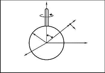
about its polar axis. Spherical polar coordinate system (~r ,θ ,ϕ )

 ~r 2 s∇nθ 

 ~r s∇nθ 
 ~r s∇nθ 
with its origin at the center of the sphere and the line θ = 0 as
Taking the divergence of (2) then substituting in (1b), we get
 ∇ ∇ 
the polar axis is adopted to describe the mathematical formu-
ρ (v ⋅ ∇v) = −∇p + 2η ∇ ⋅ d − ∇ ⋅  λ τ − 2η λ d  . (5)

~ ~

lation, Fig. 1. It is assumed that, the sphere is kept at constant

~ ~ ~ ~

o  1

o 2 

~ ~  

temperature T1 , while the fluid is still maintained at T2
with
Let the radius of the sphere, R, and the angular velocity, Ω,

~ ~

T1 > T2 . The fluid has a density ρ , heat capacity per unit mass
c p , and thermal conductivity k.
be reference values of length and velocity, respectively. Then
nondimensional variables can be defined via:

~r ~ ψ

v p 

r = , ∇ = R∇ , Ψ = , R R3 Ω

V = , RΩ

P = , 

η o Ω 

z ~ ∇ ~ ∇

~ ~ 

(6)

τ ∇ τ

d ∇ d

T − T2 

τ = , τ =

Ω η Ω

2 , d =

, d =

2 , T = ~

~ .

o η o Ω Ω Ω

T1 − T2 

~ u Introducing the above dimensionless quantities into (2), (4), (5)

r υ and (1c), we get

R θ  ∇ ∇ 
~ τ = 2d − De τ − 2ξ d  , (7a)

T1 


 Ψ 

O y V ⊥ = Uˆr + Vθˆ = −∇ ∧ 

 r s∇n θ

ϕˆ  , (7b)



Fig. 1. Flow geometry.

∇ 2 V − Re Γ − De Λ − ∇P = 0 , (7c)

Pr Re V ⋅ ∇T = ∇ 2T , (7d)

where the two vectors Γ and Λ are given by:
Γ = V ⋅ ∇V , (8a)
 ∇ ∇ 
The equations governing steady, incompressible, and vis-

Λ = ∇ ⋅ τ − 2ξ d  . (8b)

coelastic flow are continuity, momentum, and energy equa-  
tions
∇~ ⋅ v = 0 , (1a)
and

ξ = λ2 . Equations (7) are characterized by Deborah num-

λ1

ρ ( v ⋅ ∇~ v)= −∇~ p + ∇~ ⋅τ~ , (1b)

ber De, Reynolds number Re and Prandtl number Pr given by:

~ ~ ~ 2 ~

ρR2 Ω

cpηo

ρ c p v ⋅ ∇T = k∇ T , (1c)

De = λ1Ω ,

Re = ,

η o

= . (9)

here v is the velocity vector, p is the pressure, T
is the tem-
Since

V = V ⊥ + Wϕˆ ,

Γ = Γ ⊥ + Γ3ϕˆ

and

Λ = Λ ⊥ + Λ3ϕˆ

with

perature of the fluid and τ ~ is the stress tensor which is given

V ⊥ = Uˆr + Vθˆ ,

Γ ⊥ =

Γ1ˆr +

Γ 2θˆ

and

Λ ⊥ = Λ1ˆr + Λ2θˆ , then

from Oldroyd-B model [20], [21] as:

∇  ∇

(7c) may be decomposed into the ϕ -component and the vector equation including the r- and θ -components as:

τ + λ 1

τ = 2η

 d + λ




d  , (2)




∇ 2 (Wϕˆ )− (Re Γ3 + De Λ3 )ϕˆ = 0 , (10a)

where d
is the rate of strain tensor, λ 1 is the relaxation time,
∇ 2 V

⊥ − Re Γ

⊥ − De Λ ⊥

− ∇P = 0 . (10b)

λ2 is the retardation time, η o is the zero-shear rate viscosity and the symbol “ ∇ ” over any tensor denotes the upper- convected derivative. Setting λ2 = 0 in (2) reduces it to Max-

Applying the curl operation to (10b) and using (7b), the equa- tions of motion, (10a) and (10b), after some mathematical han- dling are reduced to:
well model while Newtonian fluid is obtained by setting
1 

∂ r

(r 2 W ,

)+ ∂  1 ∂

(W s∇nθ )  − Re Γ

− DeΛ3
= 0 (11a)

λ 1= λ2 = 0 .

In spherical polar coordinates, the velocity field and the

r 2 

 s∇nθ  

=s∇n  

∂2 +

θ ∂  1


∂  Ψ − Re s∇nθ ∂ rΓ
− ∂ Γ
temperature may be written as:

~ ~

 r r2

θ  s∇nθ θ 

[ r ( 2 )

θ 1]

v = [u(~r ,θ ) , υ(~r ,θ ) , w(~r ,θ )],

T = T(~r ,θ ) , (3)

− θ [∂ ( Λ ) − ∂ Λ ] = 0
the velocity and the temperature are independent of the coor-

De s∇n

r r 2 θ 1

(11b)
dinate ϕ due to the symmetry about the z-axis. Since the flow is described in the meridian plane, the velocity components u
The components of Γ and Λ are given in the Appendix.

238

International Journal of Scientific & Engineering Research, Volume 6, Issue 1, January-2015 239

ISSN 2229-5518

3 BOUNDARY CONDITIONS

5.1 Creeping Flow

~ This step of approximation produces the leading terms in the

We assume that, the sphere is kept at constant temperature T1

~ ~ ~

expansion of W, Ψ and T. The solution of these terms repre-
while the fluid at infinity is still at T2
such that T1 > T2 . Also
we assume that, the sphere is rotating with angular velocity
sent the creeping flow around the rotating sphere [22]. The

Ω = Ω zˆ . The linear velocity at infinity vanishes,

v(∞) = 0 ,

lowest order in (14) are:
while at the sphere surface is

v( R) = Ω ∧ R ~ˆr = Ω R s∇nθ ϕˆ .

τ (0 ,0) = 2 d(0 ,0) , (15a)

Therefore, the boundary conditions in dimensionless form
∂

( , ) + ∂

 ∂

( , ) θ 

may be formulated as:

( 2 0 0 )  1

( 0 0

) = 0

s∇nθ 
0
1
 1 

r r W ,r

θ  s∇nθ θ W

s∇n


, (15b)

W =  0

 , Ψ =Ψ ,r =   , T =   for

r = 

 , (12a) 

s∇nθ

  Ψ
  0
0
∞

∂ 2 +

r 2

∂θ 
1 ∂ 

s∇nθ θ 

( 0 ,0) = 0

, (15c)

and the symmetry conditions at the poles, (θ = 0, π ) , are: 

 
with the boundary conditions:
0
W =Ψ =Ψ ,r = T =  
for
 0 

θ = π  . (12b)

W ( 0 ,0)

= s∇nθ , 0 and

Ψ ( 0 ,0) =Ψ

,( 0 ,0) =

0, 0
for r = 1, ∞ . (15d)
0  
The solutions of (15b) and (15c) which satisfies the boundary conditions are:

4 THE METHOD OF SUCCESSIVE APPROXIMATION

The solution of the problem is obtained by the perturbation method. The perturbation parameters that describe the im-

W ( 0 ,0) = s∇nθ

r 2

and
, (16a)
portance of the inertial and elastic effects are the Reynolds and Deborah numbers. So, the dynamical variables are expanded as a power series in Re and De. For example, for H we write

Ψ ( 0 ,0) = 0 . (16b)

Regarding the heat transfer prediction, the coefficient of

Re0 De0 in the energy equation, (7d), shows that the function

( 0 , 0)

H = ∑Rem Den H( m, n)

T must satisfy the equatioin:

2 ( 0 ,0)

m, n=0 (13) ∇ T

= H( 0 , 0) + Re H(1,0) + DeH( 0 ,1) + Re De H(1,1) + ... or

= 0 , (17a)

2 ( 0 ,0) +2

(0 ,0) +

(0 ,0) = 0

with the help of (13), the governing equations, (7a), (11a) and

r T ,rr

rT ,r

T ,θθ

cotθ T ,θ

, (17b)
(11b) take the form:
with the boundary conditions:
  ∇ ( m,n)

∇ ( m,n) 

T ( 0 ,0) = 1, 0

for

r = 1, ∞ . (17c)

∑ Re m De n τ ( m,n) − 2d( m,n) + De τ

− 2ξ d
 = 0
The solution of (17b) and (17c) is:

m,n=0


n  1 

2 ( m,n)



 1


( m,n)

(14a)
 

T ( 0 ,0)

= 1 . (17d)

∑ Re

m,n=0

De 

 r

2 ∂ r (r



W ,r

)+ ∂θ 
 s∇nθ

( m, n)

∂θ (W

( m, n) 

s∇nθ ) 

 

5.2 Secondary Flow due to Inertial Effect

In this section, we find the secondary flow due to small iner- tial effects (centrifugal forces). Therefore, the coefficients of
− Re Γ3
− DeΛ3
 = 0 , (14b)


Re1 De0 in (14) are:

 
1  ( 2

(1,0) )

 1 (

(1,0)

)  −

( 0 ,0) = 0

∑ Rem Den ∂2 + s∇nθ ∂  1

 ( m, n) ( m, n)
 Re s∇n r

∂ r

r 2  r

W ,r

+ ∂θ  ∂θ W
 s∇nθ

s∇nθ   Γ

  3
, (18a)

m, n=0



r2 θ  s∇nθ

θ 

r 2

∂ 2


+ s∇nθ ∂  1

 (1,0)


− s∇nθ [∂

(rΓ (0 ,0)

)− ∂

Γ (0 ,0)

]= 0 ,

− ∂ Γ ( m, n) ]− De s∇nθ [∂ (rΛ( m, n) )− ∂ Λ( m, n) ]  = 0 . (14c)
 r θ

 s∇nθ θ 

r θ 1

θ 1 r 2 θ 1


(18b)
The boundary conditions, (12a), can be written as:
with
δ δ

s∇nθ 

0

W (1,0) = 0, 0

and Ψ (1,0) =Ψ ,(1,0) = 0, 0

for

r = 1, ∞ . (18c)

W ( m,n) =  m0 0n

, Ψ ( m,n) =Ψ ,( m,n) =   , r
 0 

r 0

The solution of (18) requires the determination of

( 0 ,0)

∇

for

T ( m,n) = 

m0δ 0n

,
for
1

r =   . (14d)

∇ = 1, 2,3 . Since V ( , ) = [0, 0, W ( , ) ], we get from (A.1) in the
δ   

0 0 0 0

 0 
∞

Appendix the components Γ ( 0 ,0) as:

where δ ∇j is the Kronecker delta function.

( 0 ,0)

U( 0 ,0)U ,( 0 ,0)

1 (V ( 0 ,0)U ,( 0 ,0)

Γ1 =

5 SOLUTION OF THE FLOW EQUATIONS

The solution of (7d) and (14) subject to the boundary condi-

r + θ

− V ( 0 ,0)2 − W ( 0 ,0)2  = −r−5 s∇n2 θ , (19a)


tions (14d) up to the first order, is the chief object of this paper.

Γ ( 0 ,0) = U ( 0 ,0) V ,( 0 ,0) + 1 (V ( 0 ,0) V ,( 0 ,0) +U ( 0 ,0) V ( 0 ,0) ,

The flow equations are not coupled with the energy equation 2
and need to be solved before the solution of the later one.

r r θ

239

International Journal of Scientific & Engineering Research, Volume 6, Issue 1, January-2015 240

ISSN 2229-5518

and

− W ( 0 ,0)2 cotθ  = −r−5 s∇nθ cosθ , (19b)



solution:

W ( 0 ,1) = 0 . (25)

Γ ( 0 ,0) = U( 0 ,0)W ,( 0 ,0) + 1 (V (0 ,0)W ,(0 ,0) +U(0 ,0)W (0 ,0)

Equation (22c), after substitution of Λ(0 ,0)

and Λ(0 ,0)

, reduces

3 r r

+ V ( 0 ,0)W ( 0 ,0) cotθ ) = 0 . (19c)

to:
 2

s∇nθ  1

 0 1

−7 2

Therefore, (18) take the forms:
∂ r +


∂θ 

r 2  s∇nθ

∂θ 

Ψ ( , ) = −144 (1 − ξ ) r

s∇n

θ cosθ ,

∂ (r 2W ,(1,0) )+ ∂θ 


1

s∇nθ θ

(W (1,0)

s∇nθ ) = 0 , (20a)


(26a)
the solution of this equation for the boundary conditions (22d)
is:

∂2 + s∇nθ ∂  1

 Ψ (1,0) = 6r−5 s∇n2 θ cosθ . (20b)

Ψ ( 0 ,1) = −

1 (1 − ξ ) r −3 (r − 1)2 (r + 2) s∇n2 θ

osθ . (26b)

 r r2

θ  s∇nθ

θ  c

The boundary conditions imposed on (20) implies that, the
only solution satisfying (20a) is:

W (1,0) = 0 , (21a)

From Ψ ( 0 ,1) we can obtain the components of the velocity

V ( 0 ,1)

and the solution of (20b) is:

( 0 ,1) = −1

Ψ ,θ ,1) = −

1 (1 − ξ ) r
2

−5 (r −1)2 (r + 2) (1 − 3 cos2 θ ),

Ψ (1,0) = 1 1 − 1 

s∇n2 θ

cosθ . (21b)

r s∇nθ

 
8  r 
(26c)
By taking (7b) into account, the components of the velocity

V ( 0 ,1) =

1 Ψ ,( 0 ,1) = −3(1 − ξ ) r −5 (r − 1)s∇nθ cosθ , (26d)

V (1,0)

(1,0)

r s∇nθ r

⊥ can be calculated from Ψ as:

U (1,0) =

−1 Ψ ,(1,0) = 1 r −4 (r − 1)2 (1 − 3 cos2 θ ), (21c)

and

r 2 s∇nθ θ 8

6 EFFECTS OF SECONDARY FLOW ON HEAT TRANSFER

Energy equation, (7d), is a non-linear second-order partial dif-

V (1,0) =

1 Ψ ,(1,0) = 1 r −4 (r −1) s∇nθ cosθ . (21d)

ferential equation. The density function,

V ⋅ ∇T , in its left

r s∇nθ r 4

5.3 Secondary Flow due to Elastic Effect

The coefficients of Re 0 De1 in (14) are

hand side is known from the solution of the flow equations. The secondary flow effects on heat transfer through its contri- bution to the velocity field. To find these effects due to both inertia and elastic, we solve the energy equation up to the se-

∇ (0 ,0)

τ ( 0 ,1) = 2 d( 0 ,1) − τ

∇ (0 ,0)

+ 2ξ d
(22a)
cond-order approximation.

6.1 Inertial Effects

1  ( 2

( 0 ,1) )

 1 (

( 0 ,1)

) 

( 0 ,0) 0

2 ∂ r

r W ,r

+ ∂θ  θ W

s∇nθ 

 − Λ3 =

(22b) 1 0

r   s∇nθ  

The coefficient of Re De
in (7d) is:

2 s∇nθ 1

 

 Ψ

0 1 −

θ [∂ ( Λ 0 0 )− ∂

Λ 0 0 ]= 0

(22c)

∇ 2T (1,0) = Pr V (0 ,0) ⋅ ∇T (0 ,0) , (27a)



 r r 2

∂θ  ∂

 s∇nθ



θ 

( , )

s∇n

( , )

r 2

( , )

θ 1

with the boundary conditions
with the boundary conditions

T (1,0) = 0 , 0

for

r = 1, ∞ . (27b)

W ( 0 ,1) = 0, 0 and Ψ ( 0 ,1) =Ψ ,( 0 ,1) = 0, 0 for

r = 1, ∞ . (22d)

By taking the zero-order solution into account, the right hand

The lowest order solution shows that, the non-vanishing com- ponents of τ ( 0 ,0) and d( 0 ,0) are:

side of (27a) equal to zero. So, the solution of (27a) with the
boundary conditions (27b) is:

τ ϕ,0)

d(ϕ,0) (rW ,(0 ,0)

W (0 ,0) )

r −3 s∇nθ

T = 0 . (27c)

(0 = 2 0 = 1 −

r r

= −3
(23a)

(1,0)

The coefficient of

Re 2

De0 in (7d) is:

therefore, by using (A.4) and (A.5), the non-vanishing compo-

∇ ( 0 ,0)

∇ 2T ( 2 ,0) = Pr[V ( 0 ,0) ⋅ ∇T (1,0) + V (1,0) ⋅ ∇T ( 0 ,0) ] , (28a)

nents of τ and d

are:
with the boundary conditions

∇ ( 0 ,0)

τ ϕϕ

∇ ( 0 ,0)

= 2 dϕϕ

= −18r −6 s∇n2 θ

(23b)

T ( 2 ,0) = 0 , 0

for

r = 1, ∞ . (28b)

The right hand side of (28a) can be calculated as:

while any other components are zeros. Therefore, the compo- nents of the vector Λ ( 0 ,0) appearing in (22) are given by:

V ( 0 ,0)

⋅ ∇T

(1,0)

= 0 , (28c)

Λ( 0 ,0)

ξ −7 2 θ

V (1,0) ⋅ ∇T ( 0 ,0) = U (1,0)T ,( 0 ,0) = − 1 r −6 (r −1)2 (1 − 3 cos2 θ ), (28d)

1 = 18(1 − ) r

s∇n

, (24a) r 8

Λ( 0 ,0) = 18(1 − ξ ) r −7 s∇nθ cosθ , (24b)

therefore, (28a) takes the form:
and

Λ(0 ,0) =

0 . (24c)
 (r 2 ∂
 r r

)+ 1

s∇nθ


∂θ s∇n ∂θ T =

(29a)

Since Λ( 0 ,0) = 0 , then the only solution of (22b) is the identical

− 1 Pr r −4 (r −1)2 (1 − 3 cos2 θ )
8
240

International Journal of Scientific & Engineering Research, Volume 6, Issue 1, January-2015 241

ISSN 2229-5518

the complete solution of the last equation is:
− 1 A 
2  1 2

T ( 2 ,0) =

Pr (r − 1)(3r −3 + 2r −4 )(1 − 3 cos2 θ ). (29b)

U = r 2 s∇nθ θ

= 2 1 −

r 



B1 +


  

1 

r  r 

(1 − 3 cos2

θ ), (34a)

96 and
= 1
= =2
1 − =3
 1 − =1 
. (34b)

6.2 Elastic Effect

V Ψ ,

A  B  

 s∇nθ cosθ

r s∇nθ r

r 3 

r   r 

To show the elastic effect on heat transfer due to normal
stresses, we solve the energy equation up to the first order of

Re De . So, the coefficient of this order in (7d) is:

∇ 2T (1,1) = Pr(V ( 0 ,0) ⋅ ∇T ( 0 ,1) + V ( 0 ,1) ⋅ ∇T ( 0 ,0) ) , (30a)

with the boundary conditions
The known expressions for the velocity components must be introduced in the expression of V to obtain the complete solu-
tion for the velocity field around the rotating sphere as:

V = Uˆr + Vθˆ + W ( 0)ϕˆ , (35)

As expected, the stream and velocity functions show that

T (1,1) = 0 , 0

for

r = 1, ∞ . (30b)

the flow field is under the effect of both inertial and elastic
By using (17d) and (26), the terms in the right hand side of
(30a) are given by:

V (0 ,0) ⋅ ∇T (0 ,1) = 0 , (31a)

V ( 0 ,1) ⋅ ∇T ( 0 ,0) = U ( 0 ,1)T ,( 0 ,0) =

effects. The dimensionless quantity "B" in (33b) determines the shape of the streamline and velocity profiles while "A" deter- mines their absolute values. Secondary flow is a consequence of interaction between both inertial and elastic forces. The flow pattern varies with the value of "B" as the following:

1 (1 − ξ ) r −7 (r −1)2 (r + 2) (1 − 3 cos2 θ )

2
so, (30a) takes the form:
(31b)
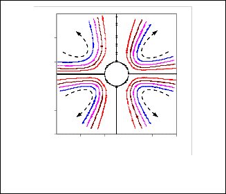
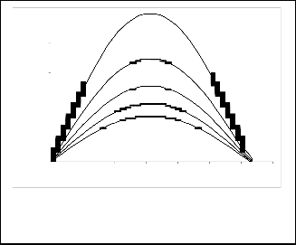
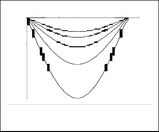
1. For B ≤ 1 , the inertial force determines the nature of flow
field as in Figs. 2a, 3a and 4a. These forces caused fluid to be thrown outward centrifugally at equatorial zone. So,
 (r 2 ∂
 r r

)+ 1 ∂

s∇nθ θ

(s∇nθ ∂θ

) T (1,1) =


(32a)
the secondary flow is directed to the inside at the poles
( θ = 0,π ) and to the outside at the equator zone ( θ = 1 π ).

Pr(1 − ξ ) r −5 (r −1)2 (r + 2) (1 − 3 cos2 θ )

2
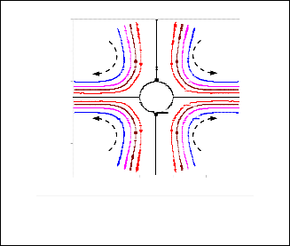
2. For

1 < B < 1 , the elastic forces dominate near the surface

the solution of this equation is:

T (1,1) = − 1 Pr(1 − ξ )(r − 1)(7r −3 − 10r −4 + 4r −5 )(1 − 3 cos2 θ ). (32b)
56

7 RESULTS AND DISCUSSION

of the sphere and further away from the sphere, the iner-
tial forces dominate the flow situation. A complete picture
of such flow situation is given in Figs. 2b, 3b and 4b.
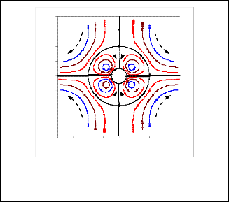
3. For B ≥ 1 , the secondary flow due to elastic forces is dom-
inate, see Figs. 2c, 3c and 4c. It is directed to the inside in
the equator zone and to the outside at the poles. The two
zones being separated by conical surface given by

7.1 Streamline and Velocity Profiles

θm∇n = cos

1 ≅ 54.75o

. This behavior is in agreement
According to the perturbation technique employed in section
(4), the solution of the boundary value problem defined by
(14c) is being:
with the flow pattern observed experimentally [12].
4. For B > 2 , the shape of the streamline and velocity profile
become independent on B, see Figs. 2d, 3d and 4d.

Ψ (r ,θ ) = ReΨ (1,0) + DeΨ ( 0 ,1) , (33a)

The primary flow, meridunal velocity

W ( 0)

in Fig. 5a, is a

which shows that, the effective secondary flow of a viscoelas- tic fluid results from the superposition of both inertia, Ψ (1,0) , and elastic, Ψ ( 0 ,1) , components. The different signs of the ex-

pressions in (21b) and (26b) show in fact that both effects have opposing tendencies in respect of the flow direction. There- fore, the properties of the resultant streamline pattern depend on the relative magnitudes of the two effects, or more accu-
rately, on the ratio of Re to De. By using (21b) and (26b), it is
pure drag flow for which every fluid point revolves in a circle whose center lies on the axis of rotation. All particles that ro- tate with the same angular velocity lie on one surface of rota- tion. So, the flow field consists of a set of rotational symmetric layers, which rotate at various angular velocities around the common axis. So, the adjacent layers slide over each other and there is an overall shear flow that results from the zero-order
possible to obtain the stream function in dimensionless form
stress component

( 0 ,0)

rϕ

, (23a). Fig. 5b shows that,

( 0 ,0)

rϕ

as:

 =2 

=1  2

reaches its maximum value on the equator zone ( θ = 2 π ) and
Ψ = A1 − B1 +
1 −

 s∇n2 θ cosθ , (33b)

vanishes at the poles ( θ = 0,π ). For shear flow, it is well

where

A = 1 Re

 r 
and

r 

4 De (1 − ξ )

B = . (33c)

known that the normal stress differences are proportional to the square of the shear rate [21]. Therefore, the fluid under the action of this normal stress difference flows inwards in the vicinity of the equator (high stress difference) and outwards at
From the definition of the stream function, (4), and by using
(33b), it is possible to obtain the individual velocity compo-
nents U and V as:
the poles (low stress difference).

241

International Journal of Scientific & Engineering Research, Volume 6, Issue 1, January-2015 242

ISSN 2229-5518

5 5

3 3

1 1

y y

-1 -1

-3 -3

-5 x

-5 -3 -1 1 3 5

-5

-5 -3 -1 1 3 5

Fig. 2a. Stream lines at

B = 0.3 . Inertial force caused fluid to be

Fig. 2d. Stream lines at

B = 3 . For

B > 2 , the shape of the

thrown outward centrifugally at the equatorial zone.

streamline become independent on B .

8 0.03

y 0

-2

-4

0.02

0.01

Inertial force efects

-6

-8

-8 -6 -4 -2 0 2 4 6 8 x

0 r

0 5 10 15 20

Fig. 2b. Stream lines at

B = 0.66 . Elastic forces dominate near

Fig. 3a. Radial velocity at

B = 0.3, θ = π 2 . For

B < 1 3 , the

the sphere surface and inertial forces dominate away from the sphere

inertial forces determine the nature of the radial velocity profiles.

5 0.01

Inertial force efects

U 0

0 5 10 15 20

-1

-0.01 r

-3 -0.02

-5

-5 -3 -1 1 3 5 x

-0.03

Elastic force effects

Fig. 3b. Radial velocity at

B = 0.66, θ = π 2 . For

1 3 < B < 1 ,

Fig. 2c. Stream lines B = 2 . Elastic force caused fluid to be thrown inward at equator zone.

elastic forces dominate near the sphere surface and inertial forces dominate away from the sphere.

242

International Journal of Scientific & Engineering Research, Volume 6, Issue 1, January-2015 243

ISSN 2229-5518

-0.04

-0.08

-0.12

-0.16

0 5 10 15 20

Elastic force effects

0.6

0.4

0.2

I2nertial forc4e efects

6 8 10

-0.2

Fig. 3c. Radial velocity at

B = 2, θ = π 2 . For

B ≥ 1 , elastic

-0.2

Fig. 4b. Azimuthal velocity at

B = 0.66, θ = π 2 . For

1 3 < B < 1 ,

forces determine the nature of the radial velocity profiles.

elastic forces dominate near the sphere surface and inertial

forces dominate away from the sphere

-0.1

-0.2

-0.3

-0.4

0 5 10 15 20

Elastic force effects

2 Elastic force effects

0 1 2 3 4 r 5

Fig. 4c. Azimuthal velocity at

B = 2, θ = π 2 . For

B ≥ 1 , elastic

Fig. 3d. Radial velocity at

B = 3, θ = π 2 . For

B > 2 , the shape

forces determine the nature of the azimuthal velocity profiles.

of the velocity profiles become independent on B .

-0.1

0 2 4 6 8

r 10

-0.2

Inertial force efects

Elastic force effects

-0.3

-0.4

0 1 2 3 4 5

Fig. 4d. Azimuthal velocity at

B = 3, θ = π 2 . For

B > 2 , the

Fig. 4a. Azimuthal velocity at

B = 0.3, θ = π 2 . For

B < 1 3 , the

shape of the velocity profiles become independent on B .

inertial forces determine the nature of the velocity profiles.

Elastic force effects

243

International Journal of Scientific & Engineering Research, Volume 6, Issue 1, January-2015 244

ISSN 2229-5518

0.8

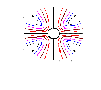
the annular region between the rotating sphere and the stag- nation surface into four similar vortices symmetric about the axis of rotation. The elastic stress effect is dominant inside, so that the same direction results as shown in Fig. 2b. The exter- nally prevailing inertia effect causes the outer vortices to ro- tate in the opposite direction.

0.6

The stagnation sphere of radius Ro
is defined as the sur-

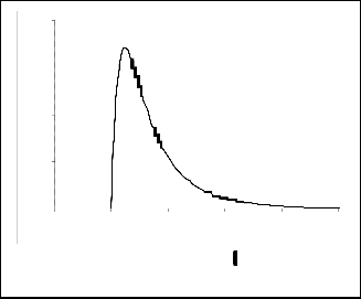
W(0)

0.4

face for which U = 0 . So by using (34a) we can calculate the
value of Ro as:

0.2

Ro =

2Bo
1 − Bo
. (37)

0 0.5 1 1.5 2 2.5 3 3.5

The effect of the stagnation surface on heat transfer process is discussed in more details in later section.

7.3 Eddy Points

The eddy points, or secondary flow centers, are defined as the

Fig. 5a. Meridunal velocity W ( ) at

B = 2 , and

points for which U = V = 0 . From (34a) and (34b) these points

r = 1, 1.2, 1.4, 1.6, 1.8 (top to bottom respectively)

are given by:
2 1 2

1 − B1 +  1 − 

(1 − 3 cos2 θ )= 0 , (38a)

    
 

and

r   r 

0 0.5 1 1.5 2 2.5 3

3.5

 =3B   1 

1 −  1 −  s∇nθ cosθ = 0 , (38b)

 r   r 

-0.5

Equation (38a) gives the radius Ro
of the stagnation surface.
Fig. 6 shows that, the eddy points are formed in the interior of

-1

the fluid between
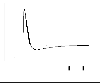
1 < r < Ro . So, it may be calculated from

τ (0, 0) -1.5

(38a) and (38b) that, if an eddy point exists, it may lie either on
θm∇n = cos

-2

1 3 ≅ 54.75o ,

1 − 3cos2

θ = 0 , or on a circular

streamline r = Rc = 3Bo
for which V = 0 , see the red circle in

-2.5

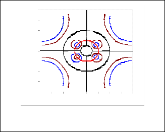
Fig. 6. So, the coordinates of any eddy is (3B , 54.74o ).

-3

Fig. 5b. Stress tensor component τ (0,0) at B = 2 , and

r = 1, 1.2, 1.4, 1.6, 1.8 (bottom to top respectively)

4 Ro

7.2 Stagnation Stream Surface

It is clear that, the properties of the resultant stream line pat- tern depend on the numerical value of the parameter B. From (9) and (33c), we can write the parameter B as:

B = 4(λ1 − λ2 )ηo . (36)

ρR2

Note that this parameter apart from the physical properties (ρ, ηo ,

y 0

-2

-4

-6

-8 x

-8 -6 -4 -2 0 2 4 6 8

λ 1 and λ 2 ), depends only on radius of the sphere R, but not on its

rate of rotation. Therefore, for a given viscoelastic fluid, the flow pattern can only be affected by the size of the rotating sphere.

Fig. 6. Stagnation stream surface and eddy points

If the parameter B = B where B has its value between 1
From the temperature point of view, the circular streamline
of radius

Rc = 3Bo

divides the annular region between the

and one ( 3 < Bo < 1 ) which can always be obtained by a

solid sphere,

r = 1 , and the stagnation surface,

r = Ro

, into
suitable sized sphere, then a spherically shaped stagnation

stream surface occurs in the fluid. As shown in Fig. 2b; the stream line of the normalized stream function Ψ (r ,θ ) divides

two concentric parts. The inner region in the range 1 < r < Rc
represents a temperature suction region in which the rotating

244

International Journal of Scientific & Engineering Research, Volume 6, Issue 1, January-2015 245

ISSN 2229-5518

eddy absorb the temperature from the heated solid sphere and then inject it to the outer region in the range Rc < r < Ro .

7.4 Heat Transfer Results

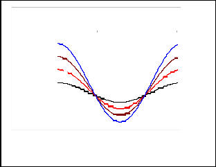
As we have seen in the previous sections, the flow depends on Re and De while the temperature distribution depends on Re, De and Pr. The solution of the energy equation is given by:

-0.0618

-0.062

0 1 2 3

Pr = 0.8

Pr = 0.6

T = T (0 ,0) + Re 2 T ( 2 ,0) + Re De T (1,1) . (39a)

The zero- and the higher-orders solution of the energy equa-
tion are given by (17d), (29b) and (32b) respectively. So, the resultant temperature is given by:

T = r −1 + 2 A 2 Pr (r −1) [7(3r −3 + 2r −4 )

-0.0622

Nu2

-0.0624

-0.0626

-0.0628

Pr = 0.4

Pr = 0.2

21
−3B(7r −3 −10r −4 + 4r −5 )](1 − 3 cos2 θ )
(39b)

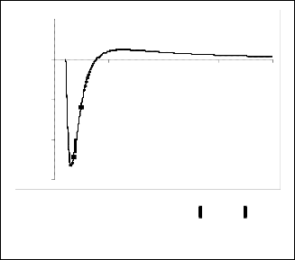
Fig. 7b. Nusselt number distributions for stagnation surface

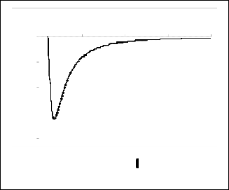
In this study, it is more convenient to work in terms of the
local Nusselt number, Nu, which can be obtained from the gradient of the temperature at the surface of the sphere and at

r = Ro at

B = 0.66 , A = 0.1 and different values of Pr.

the stagnation surface:

8 CONCLUSION

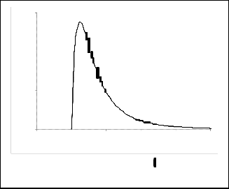
Nu1

= T ,

r r=1

= −1 + A2 Pr(35 − 3 B)(1 − 3 cos2 θ ), (40a)

The problem to be treated here is the study of the secondary flow effect on heat transfer from a rotating sphere to Oldroyd-

Nu2 = T ,

r r= Ro

= (1 − 3 cos2 θ ), (40b)
B fluid. With the help of the perturbation method, the govern-
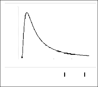
Figs. 7a and 7b show the local hemispheric Nusselt number distributions for the solid sphere and the stagnation surface

( Nu1 , Nu2 ) respectively at B = 0.66 , and A = 0.1 . At the equa-

tor, cold fluid was pulled from the stagnation surface to the solid sphere, and heat transfer from the solid sphere was at its
ing equations are splitted into two parts: creeping part, and
the deviation describing the disturbance due to inertia and elastic effects. The solution of the problem shows that, any rotation of the sphere set up a primary flow around the axis of rotation. This motion induces an unbalanced inertial and elas-
greatest. Therefore, there was a local maximum for the

Nu1

tic force fields which drives the secondary flow in the meridi-
distribution. Afterwards, fluid moving up and down to the poles along the fluid was heated gradually by the hot wall. Meanwhile, the temperature gradient in the radial direction
an plane. The secondary flow produces forced convection
within the fluid. The relative magnitudes of the secondary flow and forced convection effects depend on the parameters
and Nu1 decreased gradually forms a local

Nu1 minimum at

involved such as Reynolds, Deborah and Prandtl numbers.
the poles. By contrast, at the poles, where the stagnation sphere received heat from the hot radial outflow, heat transfer at the stagnation sphere was at its greatest, thereby forming a

9 ESTIMATION OF THE ERROR DUE TO THE SHAFT

In the absence of the shaft, the slow rotation of the sphere
local maximum at

Nu2

distribution. Fluid returning to the
about the z-axis is supposed to create a laminar velocity field
equator along the stagnation sphere was then cooled gradual-
whose magnitude at the surface of the sphere is:
ly by the cold fluid. Meanwhile, the temperature gradient in

W ~r = R= Ω R s∇nθ

, (41)
the radial direction and Nu2
decreased gradually forms local
the shear stress due to this component, at the surface can be
minimal of

Nu2 at the equator.

estimated as: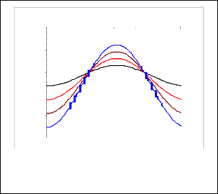

τ ~r = R= ηoW ,~r ~r = R= ηo Ω s∇nθ . (42)

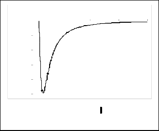
-0.96

0 1 2 3

The power required to overcome this stress in order to rotate the sphere is approximately

2π π

-0.98

P = ∫ dϕ ∫

[τ W ] ~=

R 2 s∇nθ dθ = 8 πη Ω

2 R3

. (43)

W r R 3 o

0 0

NU1 -1

-1.02

-1.04

-1.06

Pr = 0.2

Pr = 0.4

Pr = 0.6

Pr = 0.8

This power is responsible for the torque acting on the sphere surface.
In the presence of a cylindrical shaft, an additional velocity field is created due to its rotation. The tangential velocity component of this field in the neighborhood of its surface is:

∗

W = Ω Rs , (44)

where

Rs is the radius of the shaft, see Fig. 8. Similarly, the

Fig. 7a. Nusselt number distributions for the solid sphere

stress created by this field requires an amount of power to

r = 1 at

B = 0.66 , A = 0.1 and different values of Pr.

rotate the shaft. This power is of magnitude

245

International Journal of Scientific & Engineering Research, Volume 6, Issue 1, January-2015 246

ISSN 2229-5518

∗ 2π Ls ∗ ∗

1  3  ∇

∇  1

  ∇

∇ 

2 2 2

Λ2 =

∂ r r

τ rθ − 2ξ d rθ  + ∂θ s∇nθ τ θθ − 2ξ dθθ 

r s∇nθ

P W = ∫ dϕ ∫

0 0

[τ W ] ~r =R R

s∇nθ dθ = 2πη o Ω

Rs Ls . (45)

r 3  

   

cot θ ∇ ∇ 

The error caused by the shaft can be estimated as the ratio

− τ ϕϕ − 2ξ dϕϕ 

∗

P 3R2 L

r  

W = s s . (46)

Λ = 1 ∂  3  ∇

∇

− 2ξ

 1 

 + ∂

 ∇ ∇ 

θ  − 2ξ  .

PW 4R3

3 r3

r r



τ rϕ



drϕ 



r s∇n2 θ

θ s∇n



τ θϕ



dθϕ 



Thus, using a shaft of much smaller radius than R may reduce
this error. For example, let the radius of the sphere be

The components of the tensors d ,

∇ ∇

d and τ which are need-

R = 2.4 Cm . If the radius of the shaft is 0.16 Cm, and its length

(under the fluid surface) is Ls = 0.5Cm , then
ed for calculating the components of the vector Λ are:
(i) Components of d (A.3)

∗

P 3 (0.16)2

W =

(0.5) ≤ 6.94 × 10 −4 . (47)

drr = U ,r ,

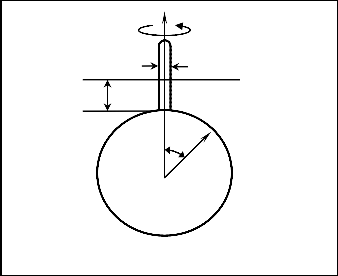
PW 4 (2.4)3

d = 1 (U + V , ),

Ω dϕϕ =

(U + V cotθ ) ,

2Rs

Fluid surface

drθ

= dθr

= 1 (U ,

2r θ

+rV , r

−V ),

Ls drϕ

= dϕr

= 1 (rW , −W ),
2r r

dθϕ = dϕθ =

(W ,θ −W cotθ ) .

∇

(ii) Components of

d (A.4)

∇

drr = Udrr ,r + r

∇

−1Vd − 2d d − 2r

−1

−1U ,θ d ,

−1

dθθ = Udθθ ,r + r

∇

Vdθθ ,θ − 2dθθ dθθ − 2r

−1

(rV ,r −V )drθ ,

Fig. 8. Error due to the shaft

dϕϕ = Udϕϕ ,r + r

Vdϕϕ ,θ − 2dϕϕ dϕϕ − 4drϕ drϕ − 4dθϕ dθϕ ,

∇

drθ = Udrθ ,r + r

Vdrθ ,θ + dϕϕ drθ − r

(rV ,r −V )drr − r

−1U ,θ dθθ ,

10 APPENIX

∇

d rϕ = Udrϕ ,r + r

Vdrϕ ,θ + dθθ drϕ − 2drϕ drr

The components of the two vectors Γ and Λ defined by (8a)

and (8b) are given by the following equations:

∇

− 2dθϕ

−1

drθ

− r −1U ,θ

dθϕ ,

(i) Components of Γ

dθϕ = Udθϕ ,r + r

Vdθϕ ,θ + drrdθϕ − 2dθϕ dθθ

Γ = V ⋅ ∇V = Γ1ˆr + Γ 2θˆ + Γ3ϕˆ , (A.1)

− 2d d

− r−1(rV , −V )d .

where
Γ1 = ˆr ⋅ Γ = UU , +

(VU ,

−V 2 − W 2 ) ,

rϕ rθ

∇

r rϕ

r r θ

(iii) Components of

τ (A.5)

Γ 2 = θˆ ⋅ Γ = UV ,r +
1 2

VV ,θ +UV − W

cotθ ),

∇

τ rr = Uτ rr ,r + r

Vτ rr ,θ − 2drrτ rr − 2r

−1U ,θ τ ,

1
Γ3 = ϕˆ ⋅ Γ = UW ,r +

(VW ,θ +UW + VW cotθ ) .

∇

τ θθ = Uτ θθ ,r + r

Vτ θθ ,θ − 2dθθ τ θθ − 2r

(rV ,r −V )τ rθ ,

(ii) Components of Λ

∇

τ ϕϕ = Uτ ϕϕ ,r + r

Vτ ϕϕ ,θ − 2dϕϕτ ϕϕ − 4drϕτ rϕ − 4dθϕτ θϕ ,

 ∇ ∇ 

∇

τ rθ = Uτ rθ ,r + r

Vτ rθ ,θ + dϕϕτ rθ − r

(rV ,r −V )τ rr − r

−1U ,θ τ θθ ,

Λ = ∇ ⋅ τ − 2ξ d  = Λ1ˆr + Λ2θˆ + Λ3ϕˆ , (A.2)

 
where

∇

τ rϕ = Uτ rϕ ,r + r

∇

Vτ rϕ ,θ + dθθ τ rϕ − 2drϕτ rr − 2dθϕτ rθ − r

−1U ,θ τ θϕ ,

1 

2  ∇

∇  1   ∇

∇ 

τ θϕ

= Uτ

θϕ ,r

+ r −1Vτ

θϕ ,θ

+ drrτ θϕ

− 2dθϕτ θθ

− 2drϕτ rθ

Λ1 = 2 ∂ r r

τ rr − 2ξ d rr  + ∂θ s∇nθ τ rθ − 2ξ d rθ 

r s∇nθ

  
1  ∇
 

∇   ∇



∇ 

−r −1 (rV ,

−V )τ rϕ .

− τ θθ + τ ϕϕ  − 2ξ  dθθ + dϕϕ 

r 

  

246

International Journal of Scientific & Engineering Research, Volume 6, Issue 1, January-2015 247

ISSN 2229-5518

11 ACKNOWLEDGMENT

The author, S. E. E. Hamza wish to thank Prof. Dr. A. Abou-El Hassan, Prof. of physics, Faculty of Science, Benha University, for his helpful guidance and valuable comments.

12 REFERENCES

[1] M.B. Bush, "The stagnation flow behind a sphere," J. Non- Newtonian Fluid Mech., vol. 49, no. 1, pp. 103, 1993.

[2] C. Bodart, and M.J. Crochet, "The time-dependent flow of a vis- coelastic fluid around a sphere," J. Non-Newtonian Fluid Mech., vol. 54, pp. 303, 1994.

[3] M.D., Chilcott, and J.M. Rallison, "Creeping flow of dilute pol- ymer solutions past cylinders and spheres," J. Non-Newtonian Fluid Mech., vol. 29, pp. 381, 1988.

[4] M.T. Arigo, and G.H. McKinley, "The effects of viscoelasticity on the transient motion of a sphere in a shear-thinning fluid," J. Rheol., vol. 41, no. 1, pp. 103, 1997.

[5] M.T. Arigo, and G.H. McKinley, "An experimental investigation

of negative wakes behind spheres settling in shear-thinning vis- coelastic fluid," Rheol. Acta, vol. 37, pp. 307, 1998.

[6] E.S. Asmolov, and J.B. McLaughlin, "The internal lift on an oscil- lating sphere in a linear shear flow," International J. Muliphase Flow, vol. 25, no. 4, pp. 739, 1999.

[7] R.S. Alassar, and H.M. Badr, "Oscillating viscous flow over a sphere," Computers and Fluids, vol. 26, no. 7, pp. 661, 1997.

[8] M. Reiner, Am. J. Math., vol. 67, pp. 350, 1945.

[9] K. Weissenberg, Proc. 1st. Intern. Congr. Rheology, vol. 3, North

Holland Publishing Co., Amsterdam, pp. 36, 1949.

[10] J.L. Ericksen, Quart. Appl. Math., vol. 14, pp. 318, 1956.

[11] J.L. Ericksen, and R.S. Rivilin, J. Rat. Math. Anal. vol. 4, pp. 323,

1955.

[12] H. Giesekus, "Some secondary flow phenomena in general vis- coelastic fluids," Proceedings of the Fourth International Congress on Rheology, Wiley-Interscience, New York, vol 1, pp. 249, 1965.

[13] J.D. Ferry, "Viscoelastic properties of polymer," Wiley, New York,

1980.

[14] I. Proudmann, and J.R.A. Pearson, "Expansions at small Reyn- olds numbers for the flow past a sphere and a circular cylinder," J. Fluid Mech. vol. 2, pp. 237, 1957.

[15] P.L. Rimmer, "Heat transfer from a sphere in a stream of small

Reynolds number," J. Fluid Mech. vol. 32, pp. 1, 1968.

[16] P.L. Rimmer, "Heat transfer from a sphere in a stream of small

Reynolds number," Corrigend. J. Fluid Mech. vol. 35, no. 4, pp.

827, 1969.

[17] S.C.R. Dennis, J.D.A. Walker and J.D. Hudson, "Heat transfer from a sphere at low Reynolds number," J. Fluid Mech. vol. 60, pp. 273, 1973.

[18] H.S. Takhar and M.H. Whitelaw, "Higher order heat transfer

from a rotating sphere," Acta Mech. vol. 30, pp. 101, 1977.

[19] M.H. Whitelaw, "Asymptotic problems in convection and vorti- ces," PhD. Thesis, Manchester Univ., 1974.

[20] R.B. Bird, and J.M. Wiest, "Constitutive equations for polymer liquids," Annual Rev. Fluid Mech. vol. 27, pp. 169-193, 1995.

[21] R.B. Bird, R.C. Armstrong, and O. Hassager, Dynamics of Poly- meric Liquids, 2nd Edn., vol. 1, Wiley, New York, 1987.

[22] W.E. Langlois, Slow viscous flow, The Macmillan Company, New

York, 1964.

247