International Journal of Scientific & Engineering Research, Volume 4, Issue 7, July-2013 1046
ISSN 2229-5518
Source Localization Wireless Sensor Network
Using Time Difference of Arrivals (TDOA)
IMRAN MEMON1 ,DEEDAR ALI JAMRO2 , FARMAN ALI MANGI3 , MUHAMMAD ABDUL BASIT4, MUHAMMAD HAMMAD MEMON5
Abstract
Source localization is a significant application of W ireless sensor networks (W SNs). Several kind of sensors can used for source localization,
such as range sensors, bearing sensors and time-difference-of-arrival (TDOA) based sensors. Time difference of arrival (TDOA) technology has been widely used in positioning and navigation system recently. The position estimation of a source through determining time difference of arrival (TDOA) of its signal among distributed sensors has many applications in civil as well as in military. In this research paper we analyses the performance of TDOA localization technique for Binary phase shift keying (BPSK)signals, the whole scenario for source localization using time-difference-of-arrival (TDOA) measurements was considered. The cross-correlation among arbitrary sensors is used to estimate TDOA also by exploiting the spectral characteristic of the received signals by considering the maximum likelihood generalized cross correlation (ML-GCC) the source will as unknown position emitting BPSK signal corrupted by the white Gaussian noise, then the weighted least square Chan’s and Taylor series methods are developed for location estimate with arbitrary sensors. W e addressed the problem is source localization via time-difference of arrival estimation in a multipath channel. Solving this localization problem typically implies cross-correlating the noisy signals received at pairs of sensors deployed within reception range of the source and solve the localization problem when there are errors in sensor positions. Correlation-based localization is severely degraded by the presence of multipath. In Simulation results show us that the proposed method for TDOA can achieve the Cramer-Rao lower bound (CRlB) accuracy compared with changing the sampling frequency of the signal and also show that the proposed method achieves a significant performance improvement over existing methods.
.
Index Terms: WLS Chan’s algorithm, CRLB, microphone array, time difference measurement, time difference of arrival (TDOA), Wireless sensor
network (WSN) ,GCC.
—————————— ——————————
1. Introduction
A continuous research and development of source localization has led to achieving more precise and accurate solution to find the true position of an emitting device in the various applications for civil and military fields.
According to civil aspects, the Sensor networks are
becoming increasingly popular for applications such as determining the position of the source of wireless
1School of Computer Science and Engineering, University of
Electronic Science & Technology
Chengdu, Sichuan 611731,China
smartimran86@yahoo.com
2 School of Physical Electronics, University of Electronic Science & Technology
,Chengdu, Sichuan 611731 ,China
deedar.jamro@salu.edu.pk
3 School of Physical Electronics, University of Electronic Science
& Technology
Chengdu Sichuan ,611731 ,China
farmanali29@yahoo.com
4School of Communication & Information Engineering , University of Electronic Science and Technology, Chengdu
Sichuan 610054 basit_266@hotmail.com
5School of Computer Science and Engineering, University of
transmission, determining the location of an acoustic source by using microphone array [1]. We determining position of a mobile receiver with pre-knowledge of transmitting time and global positioning system (GPS) [2] usually provide worldwide high accuracy position measurement. It requires to line of sight multiple satellites. Time difference of arrival (TDOA) measurements, as they are called, is also used in locating cell phones [3]. According Military aspects , the electronic warfare where the problem is to accurately locate enemy transmitters to be able to make appropriate countermeasures, the TDOA approach may here offer higher accuracy than classical localization approaches , where the TDOA measurement have larger accuracy than triangulation measurement. Source localization can be based on time of arrivals (TOA), time difference of arrivals (TDOA) or angle of arrivals (AOA) or combination of them. When the source and receiver are moving or one of them is moving so the frequency difference of arrivals (FDOA) can be exploited to improve location accuracy. In the next paragraph, some techniques will be introduced; they are used to achieve solutions for problem source localization [4].
To estimate the Direction of Arrivals (DOA) algorithms are used that exploit the phase differences or other signal
Electronic Science & Technology Chengdu, Sichuan 611731,China muhammadhammadmemon@yahoo.com
IJSER © 2013 http://www.ijser.org
International Journal of Scientific & Engineering Research, Volume 4, Issue 7, July-2013 1047
ISSN 2229-5518
characteristics between closely spaced antenna elements of an antenna array and employ phase-alignment methods for beam/null string [5, 6, and 7]. The spacing of antenna elements within the antenna array is typically less than half wavelength of all received signals. This is required to produce phase differences on the order of π radians or less to avoid ambiguities in the DOA estimate. The resolution of DOA estimates improves as baseline distances between antenna elements increase. However, this improvement is at the expense of ambiguities. As a result, DOA estimation methods are often used with short baselines to reduce or eliminate the ambiguities and other times with long baselines to improve resolution. Although, the DOA methods offer practical solution for wireless position location, they have certain drawbacks. For example accurate DOA estimates, it is crucial that the signals coming from the source to the antenna arrays must be
There are certain problems that this method could face. The estimate of the response delay within the source might be difficult to determine in practice. The main reason would be the variations in the designs of the handsets from different manufacturers. Secondly, this method is highly susceptible to timing errors in the absence of LOS, as there would be no way to reduce the errors induced because of multiple signal reflections on the forward or the reverse link.
The system that uses Time Difference of Arrivals (TDOA) to find a source location it requires at least three sensors one of them is a master (reference) and the other two are slave (Auxiliary) sensors [8, 9].
The principle of this system to measure the time difference of an intercept signal arriving slave sensor and the reference one for more details TDOA systems basically solve the equation velocity times time equals
coming from the Line-Of-Sight (LOS) direction. Another
distance,
v .t = d
, or more specifically, v δ t = δ ,
factor is the considerable cost of installing antenna arrays.
The position location system may need regular calibration
where δ t =
(t i
− t ) is the difference between the arrival
since a minute change in the physical arrangement of the array because of storms may result in considerable position location error as absolute angular position of the array is used as a reference to the angle of arrival (AOA) estimates. This is problem that would be unique to position location as this will not affect the interference rejection capability of the array. Hence, if the arrays are to be used for position location they would either need extremely rugged installation or some other method of continuous calibration for accurate DOA estimates. Another problem with this method is the complexity of the DOA algorithms. Although, there are some exceptions such as ESPIRIT and MUSIC based on Eigen value decomposition (EVD), these algorithms usually tend to be highly complex because of the need for measurement, storage and usage of array calibration data and their computationally intensive nature. It may be possible for the sensors to indirectly determine the time that the signal takes from the source to the receiver on the forward or the reverse link. This may be done by measuring the time in which the source responds to an inquiry or an instruction transmitted to the mobile from the base station. The total time elapsed from the instant the command is transmitted to the instant the source response detected, composed of the sum of the round trip signal delay and any processing and response delay within the emitting unit. If the processing delay for the desired response within the emitter is known with sufficient accuracy, it can be subtracted from the total measured time, which would give us the total round trip delays. Half of that quantity would be an estimate of the signal delay in one direction, which would give us the approximate distance of the mobile from the sensor. If the emitter can be detected at two additional receivers then the position can be fixed by the triangulation method [7].
time τ i at sensor (i)and the source time t, and δℓ is the
distance between the measurement location (x i , y i ) and source location (x , y ). After that two curves (ns-1) curves, where (ns) the number of sensors) is obtained, the point of intersection of the curves is the location of emitter some previous work had used Hyperbolic location theory to evaluate curves, the hyperbola is the set of points at a constant range difference from two foci and each sensor
pair gives a hyperbola on which the emitter lies then
emitter location estimation is the intersection of all hyperbolas.
In addition the sensors in simplified case arranged linearly or are distributed arbitrary in complex cases. Large number of sensors achieves high accuracy and performance for location estimation with more complexity of calculations.
Most researchers work to developed, they modify algorithms that used to find an emitter position estimate that minimize its deviations from the true position. We are solving the problem the reliable and accurate position location of cell phones in mobile communication.
2. Related Work:
There are several different techniques to proposed source localization methods in time-difference-of-arrival (TDOA) measurements. Y.T. Chan et al. first purposes observe the use of two spatially separated receivers to resolve the presence of a distant signal source and its relative bearing [10]. Guosong Zhang et al. purposed passive-phase conjugation uses a channel probe signal transmitted prior to the data signal in order to estimate the channel response
IJSER © 2013 http://www.ijser.org
International Journal of Scientific & Engineering Research, Volume 4, Issue 7, July-2013 1048
ISSN 2229-5518
and multipath channel, there are paths that undergo incoherent scattering by the sea surface, and they decrease the coherence between the estimated channel response and the channel response for data signal[11]. Shuanglong Liu et al purpose the analyzes the basic principle of acoustic source localization using time differe nce of arrival ,Time difference measurement is a key problem in TDOA location method for its accuracy directly determines the position estimation accuracy of the location system. Generalized cross-correlation (GCC) method can weaken the impact of noise on the delay estimation accuracy so this method is adopted in his paper to obtain TDOA measurement by detecting the peak position of the correlation function of two signals. An improved Taylor algorithm with 10 iterations is proposed to solve the location coordinate of the acoustic source[12] . Enyang Xu et al purpose he investigate robust and low complexity solutions to the problem of source localization based on the time- difference of arrivals (TDOA) measurement model. By adopting a min-max approximation to the maximum likelihood source location estimation and he develop two low complexity algorithms that can be reliably and rapidly solve through semi-definite relaxation [13].
3. System Model and its Techniques
The TDOA estimation methods will be explained in more details and discusses different algorithms that are used to estimate the time Difference of arrivals and to solve the resulting hyperbolic equations. We compare those algorithms that can be used in communication and radar systems. We measures used to measure the accuracy of TDOA estimation and introduce the measure of accuracy used throughout in this paper work.
3.1 Position Location based on TDOA Method
Hyperbolic position location (PL) estimation is accomplished in two stages. The first stage involves estimation of the TDOAs of the signal from a source, between pairs of receivers through the use of time delay estimation techniques conventional cross correlation CC and Generalized cross correlation GCC will be used to achieve high resolution TDOAs estimation when the white Gaussian noise is effected the source signal . In the second stage, the estimated TDOAs are transformed into noisy range difference measurements between sensors, resulting in a set of nonlinear hyperbolic equations. The second stage efficient algorithms to produce an unambiguous solution to these nonlinear equations. The solution provided by these equations results in the estimated
position of the source. The following is a survey of different techniques that are used to estimate the TDOAs. After that is a similar survey of the techniques and algorithms that have been proposed to accurately solve the nonlinear hyperbolic equations.
3.2 TDOA Estimation Techniques
The TDOA of a signal can be estimated by two general methods: subtracting time of arrivals TOA measurements from two base stations to produce a relative time difference of arrivals TDOA or through the use methods based on cross-correlation techniques, in which the received signal at one sensor (the reference) is correlated with the received signal at another sensor[14,15,16,17].The first method applicable if the absolute TOA measurements are available, there doesn't seem to be any advantage in converting TOA measurements into TDOA measurements, as we can triangulate the position of the source using the TOA measurements directly. However, this may give us some increased accuracy when errors due to multiple signals reflection in pairs of TOA measurements are positively correlated because of having a common signal reflector. The more similar errors in pairs of TOAs if they are more we can gain by changing them into TDOAs. However, this is practical only when we can estimate the TOA by having knowledge of transmission time. If we have no timing reference at the transmitter such as the Electronic warfare (EW) applications, then this method for estimating TDOAs cannot be used because of the absence of a timely reference on the source-to-be-located, the most commonly used technique for TDOA estimation is the cross- correlation based methods. The time requirement for this method is synchronization of all receivers participating in the TDOA measurements, which is more practical to achieve in most position location applications because of these factors we will discuss in details the cross- correlation technique for estimating TDOAs as well as the generalized cross-correlation methods.
3.3 Cross-Correlation (CC) Technique
Cross-Correlation is a measure of similarity of signal by
another signal the autocorrelation is a special case of correlation when the measure of self-similarity of a signal with its delayed version considers. Cross correlation (CC) methods cross correlate preferred version of the received signals at two sensors through filters with the proper frequency response then correlated, integrated and squared. This is performed arrange a range of time shifts. τ, until a peak correlation is obtained. The time delay causing the cross-correlation peak is an estimate of the TDOA. The aim of pre-filtering is to emerge frequencies for which SNR is the highest and attenuate the noise power before the signal is passed to correlate. The choice of the frequency function is very important especially,
IJSER © 2013 http://www.ijser.org
International Journal of Scientific & Engineering Research, Volume 4, Issue 7, July-2013 1049
ISSN 2229-5518
when the signal has multiple delays resulting from a multipath environment. If delays of the signal are not sufficiently separated, the spreading of the first multipath component function will overlap the second and another, therefore making the estimation of the peak and TDOA hardly. The frequency function might be chosen to ensure a large peak in the cross-correlation of the received signals achieving narrow band spectrum and better TDOA precision.
The signal, s (t ) , transmitting from far located radiated
source passing through a channel with interference and noise. The general model for the time-delay between receiving signals at two sensors, x1 (t) and x2 (t ), is given by
x1 (t ) = A1s (t − τ1 ) + n1 (t )
components. Many techniques have been developed that
estimate TDOA (τ) with varying degrees of accuracy.
3.4 Generalized cross-correlation:
Conventional correlation techniques that have been used to solve the problem of time difference of arrival (TDOA) estimation are referred to as Generalized Cross-Correlation (GCC) methods. These methods have been explored by Knapp [14], Allan, Azera and David [15] These GCC methods cross-correlate pre-filtered versions of the received signals at two receiving stations, then estimate the TDOA (τ) between the two stations as the location of the peak of the cross-correlation estimate. Pre-filtering is prepared to standout frequencies for which Signal-to- Noise Ratio (SNR) is low and attenuate the noise power before the signal is passed to the correlator.
x2 (t ) = A2 s (t − τ 2 ) + n2 (t )
(1)
Where A is amplitude attenuation, τ1 and τ2 are signal delayed time, n 1 (t) and n2 (t) are noise We assume that the noise is stationary white Gaussian noise and uncorrelated with signal s (t), ignoring the scaling amplitude with
consider thatτ1 >
into another form
τ 2 we could write the above equation
x1 (t ) = s (t ) + n1 (t )
x2 (t ) = s (t −τ ) + n2 (t )
Within interval


− T ≤ T ≤ T
2 2
(2)
Figure: 1 shows the block diagram of generalized cross- correlation method
Whereτ = τ1 −τ 2 , it is the desired to estimate difference
time τ the time difference of arrival between to sensors, T
The argument t that maximizes provides an estimate of the
TDOA τ. equivalently, can be written
∞
is a finite observation time, and the following assumptions hold:
R x x (τ ) =
∫s (t ) s (t −τ )dt
a. The signal
s (t ) ,
n1 (t )
and
n2 (t )
−∞
are a
(4)
stationary Random process.
b. The signal assumed to be uncorrelated with
Where T represents the observation interval; the discrete formula for the above equation is obtained by summing of N samples of given by
noise n1 (t ) and n2 (t ) .
ˆx x ( )
N −1
∑
) ( )
c. The attenuation will not be considered.
R m =
1 2 N

s (m s n + m
0
(5)
The cross-correlation and auto correlation will be as,
The cross-power spectrum is obtained by taking the
R x x
(τ ) = R ss (t −τ ) + R n n
(t )
(3)
Fourier transform of cross-correlation to improve the
1 2 1 2
Accurate TDOA estimation requires the use of time delay estimation techniques that provide resistance to noise and interference and the ability to resolve multipath signal
precision of TDOA estimation, the power spectrum of signal gives the distribution of the signal power among various frequencies and shows the existence, and also the relative power and random structure of signals, it is better to pre-filter received signals passing through the filter has
IJSER © 2013 http://www.ijser.org
International Journal of Scientific & Engineering Research, Volume 4, Issue 7, July-2013 1050
ISSN 2229-5518
response
Hi ( f ) appropriates with the spectrum of the
signals and narrow band, where i=1, 2. , because of the finite observation the estimated cross-power spectral only will be obtained and then apply an inverse Fourier transform to obtain estimated cross-correlation and finally

1 / x 2 x 2 ( )
x 1x 1
estimated TDOA. As shown is the figure 2.1 each signal
ss ( )/ [
n1n1
n2 n2
x1 (t ) and

x2 (t ) are filtered through h 1 and h 2 then
correlated integrated and squared. This is performed for a range of time shift t until a peak correlation is obtained. The time delay causing the cross-correlation peak is an
G x x (f
) 1 − γ x x (f )
estimate of the TDOA τ. If the correlator is to provide an unbiased estimate of TDOA τ, the filters must exhibit the same phase characteristics and hence are usually taken to be identical filters [2, 18, and 19].when the two signals are filtered, the cross-power spectrum between the filtered outputs given by
Table: The GCC frequency function
All these frequency functions have been derived in [11] , in our research the conventional CC and Maximum likelihood (ML) GCC will be considered .The CC has
G f = H f H * f G
(f )
already explained it. In addition when the
y 2 y 1 ( )
1 ( )
2 ( )
x 1x 2
(6)
( ) *
Where (*) denotes to complex conjugate, Therefore, the
GCC given by inverse Fourier transform of (6)
∞
H f H ( f ) = 1 ,that means the weighed frequency
2
function ΨG (f)and that makes conventional CC processor,
other processors include the Roth impulse Response
R G (τ ) =
Ψ (f )G
(f )e j 2π ft df
processor, the smoothed coherence transform (SCOT),the
y 1 y 2
∫ G x 1x 2
−∞
(7)
Ekart and Hannan-Thomoson or Maximum likelihood processors (ML) .
Where Ψ𝐺 (𝑓) = 𝐻1 (𝑓)𝐻∗ (𝑓) ΨG (f
) = H 1 (f
)H * (f )
3.5 TDOA accuracy and methods performance evaluation
denotes the general frequency weighting, or filter function.
The measurement of MRSE comparing with CRLB is a
Because only an estimate of
Gx x ( f ) 𝐺�
(𝜏) can be
1 2 𝑥1𝑥2
common method to evaluate performances of TDOA
measurement , K. C. Ho. and Friedlander, Benjamin[20,
obtained from finite observation of
∞
x1 (t ) and x2 (t ) then
21 ] have been introduced the formula of CRLB for
BPSK signals and the CRLB for ML-GCC method has
Rˆ G
(τ ) = Ψ
(f )Gˆ
(f )e j 2π ft df
been driven in [14] by using the spectral Characteristic of
y 1 y 2
∫ G x 1x 2
−∞
(8)
BPSK signal that affected with white Gaussian noise have used, then the probability density function of this model becomes Gaussian ,by considering log likelihood function and doing calculations the for our model signal
in (2)
The GCC method uses filter function ΨG (f
) to remove
the effects of noise and interference, in case of using

( 1 ∫ ( x (t )−s (t ;θ )))2 dt )
narrow band signal it achieve better TDOA estimation Using GCC; here in our work BPSK signal has been considered. Table shows the GCC frequency function.
f (x (t ), 0〈t 〈L ,θ ) = ke 2σ 0
l
(9)
We usually calculate the spectral quantities using the discrete Fourier transform (DTF) or the fast Fourier transform (FFT) as have been written in the above
paragraph.
ln f (x(t), 0〈t〈L,θ ) = ln k −
1

2σ 2 ∫
(x(t) − s(t;θ )))2 dt
(10)
The CRLB is the inverse of the Fisher information matrix defined as
Processor Name | Frequency weighted function ψG (f) |
Cross-correlation | 1 |
IJSER © 2013 http://www.ijser.org
International Journal of Scientific & Engineering Research, Volume 4, Issue 7, July-2013 1051
ISSN 2229-5518
∂2 ln f
can estimate useful TDOAs measurements. The Root

J = −E ∂θ∂θ T
(11)
Mean Squared Error (RMSE) is used as the measure of
improvement. We define the RMSE as the root square of the difference between the true TDOA value and the estimated TDOA value from the definition of RMSE with considering the CRLB that described in the chapter two in
Here the desired parameter vector here TDOA instead of θ
The exact form of CRLB of BPSK signal in case of ML- GCC method introduced by [15, 21]
−1
the equation (12) .Square root of a margin between the true
TDOA with the estimate TDOA. We compare the RMSE obtained from the ML-GCC, to RMSE for conventional CC method TDOA estimation,
CRLB (τˆ) = T
∞
∫ ( 2π f )

γ 12 (f )


2
df
To study the performance of TDOA estimator the
affection of white Gaussian noise and the spectral characteristic of the signal will be considered. In
−∞ 1 − γ (f )
(12)
simulation two ways have been used in simulation to
calculate the power spectrum density PSD for BPSK
4. Experimental Results:
We describe the simulation modelling that used to obtain the results of this work; we look at our signal model, in this work we assume the narrowband BPSK signal is radiated from the source in unknown position, this signal intercept
by the sensors in arbitrary known positions figure: 2
signal and its noise component, the PSD does not concentrate in one frequency, due to the nature of a BPSK signal in the baseband, the PSD is defined as a Sinc function , the most power of signal concentrated in the major loop and the rest are small amount of power distributed in others side loops, so we ignore the infinite interval of the spectrum and focus only in the bandwidth
scenario. MATLAB is powerful engineering software that
from the −B / 2
to B / 2 that contain the most power of
used in a lot of scientific fields was used in this work. All figures are plotted and simulated with it.
To further explain the capabilities of the GCC method, in this chapter its resolution or precision performance is compared to the resolution performance of the conventional CC method in order of estimate TDOA. The major advantage of the GCC method over CC method is able to provide resistance to noise and interference and the ability to resolve multipath signal.
The designed narrowband, baseband BPSK signal that has been considered as a radiated signal from Unknown position far stationary target with normalized amplitude the parameter of the BPSK intercepted signals the following; Code frequency (baud rate) is 10 kHz, the sampling frequency sets two values 100 kHz, The actual time delay is td = 40.166545478945465e-6 sec, the time of the signal is 500 msec.
The assumption for noise will be white Gaussian noise with zero mean; our assumption does not consider
the signal where B denotes the bandwidth.
The RMSE versus signal to noise ratio SNR has been considered, the SNR arranged from -10dB to 15 dB to show the difference between two methods in low and high SNR. The performance of the ML-GCC and CC method with different SNR levels, two ways for calculating ML-GCC method has been using the first method, the weighting function and calculate the weighting function by using a direct form of the PSD of baseband BPSK signal that presented.
the significant observation is the ML-GCC method is close to the CRLB level even though the SNR is low and the noise is white Gaussian zero mean , that because to effect of weighting function that decrease the influence of noise power spectrum and interference, with increasing SNR the conventional CC converge to the ML- GCC so we can say in high SNR no need for weighing , whatever it is better to use the ML-GCC rather than conventional CC to grantee good performance when the SNR is low or high. For more prove consider the PSD of the signals.
Gx x ( f ) = Gss ( f ) + Gn n ( f )
any relative motion among sensors or between source and
G ( f ) = G
( f )e− j 2π f τ + G
( f )
sensors so we just consider the simplest scenario in our
work.
x2 x2
ss n2 n2
(13)
4.1 The performance evaluation of TDOA estimation
Methods
We apply the methods described in Chapter two to our proposed BPSK generated signal corrupted by zero mean white Gaussian noise Our goal is to see how well we
Assume that there is no correlation between signal and noise and the power spectrum of noises are equals under this assumption the magnitude square coherence from the definition in equation
IJSER © 2013 http://www.ijser.org
International Journal of Scientific & Engineering Research, Volume 4, Issue 7, July-2013 1052
ISSN 2229-5518

G ss (f )
method performance is much better than CC that due to its weighted function has strongly relative to the nature of
(G (f
) + G
(f ))2
noise and signals.
Ψ HT =

ss nn
2
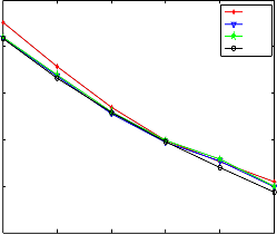
-50
hamming-TDOA estimation with the change of SNR
G (f
) 1 −

G ss (f )
CC GCC
ss
(G (f
) + G
(f ) )2
GCC-psd
ss nn
(14)
-55
CRLB
In case of SNR is high so
Gss ( f ) > Gnn ( f )
the
-60
weighting function will be
Gss ( f ) 1
-65


Ψ ( f ) ≈ =
-70
HT 2G
( f ) G
( f )
2G ( f )
ss nn nn
(15)
-75
-10 -5 0 5 10 15
SNR: dB
In case of SNR is low Gnn ( f ) > Gss ( f ) the weighting function will be
Figure: 2 shows the improvement of RMSE with increasing SNR for proposed Methods using the BT model
Ψ HT
( f ) ≈
Gss
(Gnn
( f )

( f ))2
(16)
in simulation with 200 kHz sampling frequency
rectwin-TDOA estimation with the change of SNR

-50
CC GCC
From the prove the significant results that in case when the
SNR is low and noise is Gaussian the weighting function
very sensitive so we can use the PSD of BPSK signal to
-55
GCC-psd
CRLB
weighted
G ( f )
1 2
in equation (7) and provide better
-60
estimation rather than CC method.
In case of high SNR we can use both CC and ML-GCC methods to provide good TDOA estimation as we showed in the figures.
The calculation of spectrum density functions in Matlab are replaced by two ways the first one; power Spectral Density estimate via Welch's method this method gives the PSD of signals by divided signal vector into eight sections with 50% overlap, each section is windowed with a Hamming window and eight modified period grams are computed and averaged, another method by using Blackman-Turkey BT weighted function that replaced by rectangular window in program ,the important fact that appeared in simulation results the calculation PSD via Welch method is better than BT when the SNR increase but they give same performance in low SNR, all the Results are obtained by averaging output from 400 runs simulation.
In figure 3, we observed improved of GCC with increasing sampling frequency in high SNR that may due to decreasing of spaces between samples during the processing but CC didn’t affect. Generally the ML-GCC
-65
-70
-75
-10 -5 0 5 10 15
SNR: dB
Figure 3 shows the improvement of RMSE with increasing SNR for proposed Methods using a Welch model in simulation with 200 kHz sampling frequency.
4.2 The performance evaluation of position location estimation algorithms:
To study the effect of noise on the location estimation performance, a scenario consisting of four sensors in different Geometry position was proposed, the first
IJSER © 2013 http://www.ijser.org
International Journal of Scientific & Engineering Research, Volume 4, Issue 7, July-2013 1053
ISSN 2229-5518
assumption linear fashion of sensors were considered , secondly the equally spacing geometry were considered and lastly the arbitrary distributed sensors were considered
. The measurement noise is expected to have a significant effect on the estimation accuracy; The root mean square error (RMSE) is a good technique to evaluate the performance of estimation algorithm verses the noise effect, the rise of RMSE with the noise of the Taylor - series method and Chan’s method are, Both Results are obtained by averaging output from 10000 runs simulations. The run time is another technique used to find which method is faster than another.
From the RMSE figure the significant difference here that the Taylor method has RMSE greater than RMSE for WLS Chan’s method, but for both methods the RMSE increases when the noise increases, WLS Chan’s converges to CRLB, in small amount of noise the CRLB curve that appeared in blue line and WLS Chan’s curve that appeared in a green line is seem identical but actually is not, distinguish between them is clearly shown when the Noise increases.
In figure: 5 geometrical locations of true and estimated source positions, it is clearly showed the norm distance between the actual source positions to estimate position by Taylor- series if further than that position estimated by Chan WLS methods in the following the numerical results of the proposed method will be shown as the following: Target actual position = (-1000, 3000)
Target estimation position (Taylor) =
(-997.27064 , 2999.7817)
Target estimation position (Chan's) =
(-998.00068 , 3001.3319)
Taylor estimation error = (2.7294 , -0.21829) Chan's estimation error = (1.9993 , 1.3319)
From the results generally speaking, the WLS Chan’s method is more accurate than Taylor-series. Another thing that has been observed is the running time, because of iteration the Taylor-series consuming time it needs liberalizing the set of nonlinear equation and starts from
The comparison between Chans Method & Taylor-series method of RMSE-norm
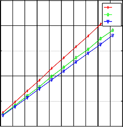
25
Taylor
Chans
CRLB
20
15
10
5
0
Figure: 4 shows the raise of RMSE when the noise variance increasing of the position estimate for proposed methods
The proposed scenario


3045

3040 
3035

3030
3025

3020
3015
3010
3005

3000
2995
the first iteration with initial guess and continue to solve and iterate until the least square error become small. For WLS Chan’s method without initial guess; the solution comes after two steps so it accesses the last solution faster than Taylor series.
-1015 -1010 -1005 -1000 -995 -990 -985
Figure: 5 shows the geometry of source actual position and the estimated position
5. Conclusion:
we presented some background information about TDOA estimation and the techniques that used to estimate TDOA measurement by subtracting TOA measurement or using correlation based methods, also we presented its applications in the real world include the civil aspects and military aspects after that; we presented different ways that used to solve the localization problems include DOA and
IJSER © 2013 http://www.ijser.org
International Journal of Scientific & Engineering Research, Volume 4, Issue 7, July-2013 1054
ISSN 2229-5518
AOA and their advantages and limitations. we presented the idea of source localization using TDOA measurement, firstly we mentioned the TDOA estimation methods based on cross-correlation, and we mentioned the conventional cross-correlation CC and Generalized cross-correlation GCC specifically the ML-GCC that used to extract and estimate TDOA measurement from the signals that radiated from far unknown position emitters ,we gave the mathematical prove of both methods and we saw the ML- GCC is strongly relatives with the spectral component of signals ,after that the position location estimation methods were presented in details the Taylor-series and Chan's WLS methods.
References:
[1]Wei Meng, Student Member, IEEE, Lihua Xie, Fellow, IEEE, Wendong Xiao, Senior Member, IEEE “Optimality Analysis of
Sensor-Source Geometries in Heterogeneous Sensor Networks”
IEEE TRANSACTIONS ON WIRELESS
COMMUNICATIONS, VOL. 12, NO. 4, APRIL 2013.
[2] CHONHOFF T A, GIORDANO A A. Detection and estimation theory and its applications [M]. Pearson College Div,
2006.
[3] Vatsal Sharan, Sudhir Kumar, Rajesh Hegde “ Multiple Source Localization using Randomly Distributed Wireless Sensor Nodes ” Communication Systems and Networks (COMSNETS), 2013 Fifth International Conference on 7-10 Jan.
2013, Bangalore.
[4] Gang Wang, Youming Li, and Nirwan Ansari, Fellow, IEEE” A Semidefinite Relaxation Method for Source Localization Using TDOA and FDOA Measurements” IEEE TRANSACTIONS ON VEHICULAR TECHNOLOGY, VOL.
62, NO. 2, FEBRUARY 2013.
[5] E. Tom Northardt, Igal Bilik, Member, IEEE, and Yuri I. Abramovich, Fellow, IEEE “Spatial Compressive Sensing for Direction-of-Arrival Estimation With Bias Mitigation Via
Expected Likelihood ” , IEEE TRANSACTIONS ON SIGNAL PROCESSING, VOL. 61, NO. 5, MARCH 1, 2013.
[6] GRAHAM A. Communications, Radar and Electronic
Warfare [M]. Wiley, 2011.
[7] WILEY R G. ELINT: The interception and analysis of radar signals [M]. Artech House Boston, 2006.
[8] FOY W H. Position-location solutions by Taylor-series
estimation [J]. Aerospace and Electronic Systems, IEEE Transactions on, 1976, 2): 187-94.
[9] CHAN Y T, HO K C. A simple and efficient estimator for hyperbolic location [J]. Signal Processing, IEEE Transactions on,
1994, 42(8): 1905-15.
[10] Chan, Y.T. “The least squares estimation of time delay and its use in signal detection, IEEE TRANSACTIONS ON ACOUSTICS, SPEECH, AND SIGNAL PROCESSING, .VOL.
ASSP-26, NO. 3, JUNE 1978.
[11] Guosong Zhang “A novel probe processing method for underwater communication by passive-phase conjugation” Signal Processing (ICASSP), 2011 IEEE International Conference on
22-27 May 2011.
[12] Shuanglong Liu “Research on acoustic source localization using time difference of arrival measurements”, Measurement,
Information and Control (MIC), 2012 International Conference on 18-20 May 2012
[13] Enyang Xu, Zhi Ding1 and Soura Dasgupta “Robust and Low Complexity Source Localization in Wireless Sensor Networks Using Time Difference Of Arrival Measurement
”, Wireless Communications and Networking Conference
(WCNC), 2010 IEEE, 18-21 April 2010, issn 1525-3511.
[14] KNAPP C, CARTER G C. The generalized correlation method for estimation of time delay [J]. Acoustics, Speech and Signal Processing, IEEE Transactions on, 1976, 24(4): 320-7.
[15] AZARIA M, HERTZ D. Time delay estimation by generalized cross correlation methods [J]. Acoustics, Speech and Signal Processing, IEEE Transactions on, 1984, 32(2): 280-5.
[16] HERTZ D. Time delay estimation by combining efficient algorithms and generalized cross-correlation methods [J]. Acoustics, Speech and Signal Processing, IEEE Transactions on, 1986, 34(1): 1-7.
[17]CARTER G C. Coherence and time delay estimation [J]. Proceedings of the IEEE.
[18] MITRA S K, KUO Y. Digital signal processing: a computer-based approach [M]. McGraw-Hill New York, 2006.
[19] VASEGHI S V. Advanced digital signal processing and noise reduction [M]. Wiley, 2008.
[20] FRIEDLANDER B. On the Cramer- Rao bound for time delay and Doppler estimation (Corresp.) [J]. Information Theory, IEEE Transactions on, 1984, 30(3): 575-80.
[21] HO K C. Modified CRLB on the modulation parameters of a PSK signal; proceedings of the Military Communications Conference Proceedings, 1999 MILCOM 1999
IEEE, 1999, 1999 .
IJSER © 2013 http://www.ijser.org