International Journal of Scientific & Engineering Research, Volume 5, Issue 5, May-2014 332

ISSN 2229-5518

Solve Boundary value problem of

Shooting and Finite difference method

Sheikh Md. Rabiul Islam

Abstract: In this paper of the order of convergence of finite difference methods& shooting method has been presented for the numerical solution of a two-point boundary value problem (BVP) with the second order differential equations (ODE’s) and analyzed. Sufficient condition guaranteeing a unique solution of the corresponding boundary value problem is also given. Numerical results are tabulated for typical numerical examples and compared with the shooting technique employing the classical Euler and fourth-order Runge-Kutta method using MATLAB 7.6.0(R2008a).

Index Terms— BVP, Shooting method, Finite difference method, MATLAB, Euler method, Runge-Kutta method.

——————————  ——————————

1. INTRODUCTION

hese problems are called two-point boundary value problems and formally have the form [1]
𝑂𝐷𝐸: 𝑦′′ (𝑡) = 𝑠�𝑥, 𝑦(𝑥), 𝑦′ (𝑥)�, 𝑥 ∈ (𝑎, 𝑏)
� (1)
𝐵𝐶𝑠: 𝑦(𝑎) = 𝛼 , 𝑦(𝑏) = 𝛽
where α and β are prescribed real values. The second order
ODE may be linear or non-linear, depending on the function
order of convergence in BVP after when 𝜖 is small

2. NUMERICAL METHOD ANALYSIS

2.1 The Euler Method

Explicit Euler’s method [1] is the simplest case of a Taylor method, where only the first term of the increment function is used, with second and higher order terms neglected.
The method is as follows:

s. The linear version of the BVP (1) is obtained by choosing

y n +1 = y n + hs(x n , y n )

(5)
the function 𝑠�𝑥, 𝑦(𝑥), 𝑦′ (𝑥)� to have a particular form,
namely

Where, s(x n

, y n

)is the source term .

ODE: 𝑦′′(𝑥) = 𝑝(𝑥)𝑦′(𝑥) + 𝑞(𝑥)𝑦(𝑥) + 𝑟(𝑥) , 𝑥 ∈ [𝑎, 𝑏
BCs: 𝑦(𝑎) = 𝛼 , 𝑦(𝑏) = 𝛽 � (2)
where the coefficients p(x), q(x) and r(x) are prescribed
functions of time, or constants. The following theorem assures existence and uniqueness of the solution of the non-linear BVP (3).
Consider the Boundary Value Problem (BVP) of the
The Euler’s method is very simple to use but accuracy can
get only first-order solution.

2.2 The Fourth Oder Runge-Kutta method

This is a popular higher order numerical method [1]. In particular, it is a fourth order accurate method whose scheme is:
ODE:𝜖𝑦′′(𝑥) + 𝑦′(𝑥) = 1; 𝑦(0) = 𝑦(1) = 0 (3)
Perform (1) applying the following methods with N = 10; 100;
1000; 10000 mesh points and damping coefficients 𝜖 =
1,0.1, 10−4 , 10−8 using Finite difference method &Shooting

y n +1 = y n + hφ ( x n , y n , h)

φ ( x n , y n , h) = 1

2(k1 + 2k 2 + 2k 3 + k 4 )

(6)
method with Euler & Runge Kutta 4th order as forward

k1 = s( x

, y n )

integrator.
The exact solution is
𝑦(𝑥) = 𝑥 − 1−exp(−𝑥𝜖 )

k = s(x n + h, y n + hk )

k = s x n + 1 h, y n + 1 hk 

1−exp(−𝜖−1 ) (4) 3  2 

The authors investigated an estimation in numerically the  2 

————————————————

Sheikh Md. Rabiul Islam, is currently pursuing Ph.D. degree program in Information science & Engineering under Faculty of Education, Science, Engineering & Technology in University of Canberra, Australia, E-mail: Sheikh.Islam@canberra.edu.au

k = s(x n + h, y n + hk )

3. SHOOTING METHOD

The shooting method begins by associating to the original
BVP (3) an IVP of the form[1]

IJSER © 2014 http://www.ijser.org

International Journal of Scientific & Engineering Research, Volume 5, Issue 5, May-2014 333

ISSN 2229-5518

𝑂𝐷𝐸: 𝑦′′ (𝑡) = 𝑠�𝑡, 𝑦(𝑡), 𝑦′ (𝑡)�, 𝑡 ∈ (𝑎, 𝑏)
𝑧 = 𝑧
+ ℎ �− 1 𝑧 + 1
� (7)

2𝑖+1

2𝑖

𝜖 2𝑖

� (19)

𝜖

𝐵𝐶𝑠: 𝑦(𝑎) = 𝛼 , 𝑦(𝑏) = 𝑔
where g is a parameter that determines an initial guess for the

slope of the curve y(t). This associated IVP (7) is solved by the

Similarly using the fourth order of Runge-Kutta method
[1];[2] we have two difference equations
𝑦𝑛+1 = 𝑦𝑛 + ℎ𝛷(𝑥𝑛 , 𝑦𝑛 , ℎ) (20)
usual methods for IVPs, we have considered the two methods
𝛷(𝑥𝑛 , 𝑦𝑛 , ℎ) = 1 (𝑘
+ 2𝑘
+ 2𝑘
+ 𝑘 ) (21)
which is Euler and fourth-order Runge-Kutta method.

• For two chosen initial slopes g1, g2 compute two solutions

2 1 2 3 4

𝑧1𝑖+1 = 𝑧1𝑖 + ℎ𝑧2𝑖 (22)

𝑛 𝑛 1 1

to IVP (7), with corresponding boundary points (g1,B(g1)) and
𝑘1 = 𝑠(𝑥
, 𝑦
) = − 𝑧 + (23)

𝜖 𝜖

(g2,B(g2)).
𝑘2 = 𝑠(𝑥𝑛 + ℎ, 𝑦𝑛 + ℎ𝑘1 ) = −


1 1 (𝑧2𝑖 + ℎ𝑘1 ) +

• Fit a straight line through the points P1 = (g1,B(g1)) and P2 =

(g2,B(g2)), namely[1]

𝐵(𝑔2 )−𝐵(𝑔1 )

𝑘3 = 𝑠 �𝑥𝑛 +
1

ℎ, 𝑦𝑛 +
2
𝜖

1
2 ℎ𝑘1 � = −

1
𝜖 �𝑧2𝑖 +
𝜖


1 1
2 ℎ𝑘1 � + 𝜖

𝐵(𝑔) = 𝐵(𝑔2 ) + �

𝑔2 −𝑔1

� (𝑔 − 𝑔2 )
𝑘4 = 𝑠(𝑥𝑛 + ℎ, 𝑦𝑛 + ℎ𝑘3 ) = −


1 1
𝜖 (𝑧2𝑖 + ℎ𝑘3 ) + 𝜖
A third value g3 is obtained by requiring B(𝑔3) = β, that is
𝑧 = 𝑧
+ ℎ 1 (𝑘
+ 2𝑘
+ 2𝑘
+ 𝑘 ) (24)

𝑔3 = 𝑔2 + �

𝑔2 −𝑔1

� (𝛽 − 𝐵(𝑔2)

2𝑖+1

2𝑖 2 1 2 3 4

𝐵(𝑔2 )−𝐵(𝑔1 )

𝑔𝑘−𝑔𝑘−1

Discretizing (15) let consider

′ = 𝑤

(25)

𝑔𝑘+1 = 𝑔𝑘 + �
� �𝛽 − 𝐵(𝑔𝑘 )�, 𝑘 = 2, … . , 𝐾. (8)

𝐵(𝑔𝑘)−𝐵(𝑔𝑘−1 )

𝑦1 = 𝑤1 𝑦1 2

′

𝑤1 = 𝑤2 𝑤1(𝑎) = 0 (26)

′ = − 1 𝑤

+ 1 , 𝑤 (𝑎) = 1 (27)

• The process is stopped if

𝑤2

𝜖 2 𝜖 2

| 𝐵(𝑔𝑘 )−β|≤TOL (9)
where TOL is a tolerance, a pre-assigned small positive real
Using the Euler method we have the two difference equations
𝑤1𝑖+1 = 𝑤1𝑖 + ℎ𝑤2𝑖 (28)
number. For single precision calculations we can take TOL =

𝑤2𝑖+1 = 𝑤2𝑖 + ℎ �−
𝑤2𝑖 +

1� (29)

𝜖

10−6.

4. NUMERICALLY SURVEY OF LINEAR SHOOTING

Similarly using the fourth order of Runge-Kutta method we have two difference equations
𝑦𝑛+1 = 𝑦𝑛 + ℎ𝛷(𝑥𝑛 , 𝑦𝑛 , ℎ) (30)

METHOD

𝛷(𝑥𝑛 , 𝑦𝑛 , ℎ) = 1 (𝑘
+ 2𝑘2
+ 2𝑘3
+ 𝑘4 ) (31)
Looking at problem class (2), we break this down into two
IVP also shown in

2

𝑤1𝑖+1 = 𝑤1𝑖 + ℎ𝑤2𝑖
1 1

′′ ′

𝑛 𝑛

𝑦1 (𝑥) = 𝑝(𝑥)y1 + 𝑞(𝑥)𝑦1 + 𝑟(𝑥) , a ≤ x ≤ b ,
𝑦1 (a) = α y′ (a) = 0 (10)
𝑘1 = 𝑠(𝑥
, 𝑦
) = − 𝑤2𝑖 +
𝜖 𝜖
1 1

′′ ′

𝑘2 = 𝑠(𝑥𝑛 + ℎ, 𝑦𝑛 + ℎ𝑘1 ) = −


(𝑤2𝑖 + ℎ𝑘1 ) +
𝑦2 (𝑥) = 𝑝(𝑥)y2 + 𝑞(𝑥)𝑦2 , a ≤ x ≤ b ,
𝑦2 (a) = 0 y′ (a) = 1 (11)
Combining these results together to get the unique solution

𝛽−𝑦1 (𝑏)

𝑘3 = 𝑠 �𝑥𝑛 +

𝑛

1

ℎ, 𝑦𝑛 +
2

𝑛

𝜖


1 1
2 ℎ𝑘1 � = − 𝜖
1
�𝑤2𝑖 +
𝜖


1 1
2 ℎ𝑘1 � + 𝜖
1
𝑦(𝑥) = 𝑦1 (𝑥) +

𝑦1 (𝑏)

𝑦2 (𝑥) (12)

𝑘4 = 𝑠(𝑥

1

+ ℎ, 𝑦
+ ℎ𝑘3 ) = −


𝜖 (𝑤2𝑖 + ℎ𝑘3 ) + 𝜖
Provided that 𝑦1 (𝑏) ≠ 0.
From the BVP of equation (3) can be written as
𝑤2𝑖+1 = 𝑤2𝑖 + ℎ (𝑘1 + 2𝑘2 + 2𝑘3 + 𝑘4 ) (32)
Combing all these to get our solution using Euler method and
1

𝑦′′ (𝑥) = −
1

𝑦′ (𝑥) +
fourth order Runge-Kutta method
𝜖 𝜖
𝑦𝑖 = 𝑧1𝑖 +

𝛽−𝑧1 (𝑏)

𝑤1𝑖 (33)
With boundary conditions 𝑦(0) = 0



𝑦(1) = 1 − 1−exp(−𝜖 )

𝑤1 (𝑏)

We divided the area into even spaced mesh points

1−exp(−𝜖−1 ) (13)

Breaking this boundary value problem into two IVP’s
𝑥0 = 𝑎, 𝑥𝑁 = 𝑏, 𝑥𝑖 = 𝑥0 + 𝑖ℎ ; ℎ =

𝑏−𝑎

𝑁

(34)
𝑦′′ = − 1

𝜖

y′ + 1

𝜖

, 𝑦1 (a) = 0 y′ (a) = 0 (14)
Wehave 𝑁 = 10,100,1000,10000 𝑎𝑛𝑑 𝑎 = 0 𝑎𝑛𝑑 𝑏 = 1 and
computation algorithm of the above is computationally
𝑦′′ (𝑥) = −

1 y′ + 1

𝜖 𝜖

, 𝑦2 (a) = 0 y′ (a) = 1 (15)

′

complex and to solve it for Shooting method using Euler and
Discretizing (14) let consider again 𝑦1 = 𝑧1 𝑦1 = 𝑧2


𝑧′ = 𝑧 𝑧 (𝑎) = 0 (16)
fourth order of Runge-Kutta method to find the hit to target
value of β with the some initial guess consider two problem
𝑧′ = −
𝑧 + 1

𝜖 𝜖

, 𝑧2 (𝑎) = 0 (17)
as shown in equation (13) and (14). In BVP of equation we
Using the Euler method we have the two difference
equations[1];[2]
𝑧1𝑖+1 = 𝑧1𝑖 + ℎ𝑧2𝑖 (18)
have also used the value of 𝜖 = 1,0.1, 10−4 , 10−8
corresponding shown Table I for Shooting method using
Euler and fourth order of Runge-Kutta method. We have also

IJSER © 2014 http://www.ijser.org

International Journal of Scientific & Engineering Research, Volume 5, Issue 5, May-2014 334

ISSN 2229-5518

tried to find the order of convergence using the equation (2) for different of N for both Euler method and Fourth order Runge-Kutta method. We have observed in Table. I when
𝜖 = 1 the error has gradually decreased as well as the order
of convergence has decreased within the mesh size increased
Since the values of 𝑝(𝑥𝑖 ) , 𝑞(𝑥𝑖 ) 𝑎𝑛𝑑 𝑟(𝑥𝑖 ) are known it
represents linear algebraic equation
involving𝑦(𝑥𝑖+1 ), 𝑦(𝑥𝑖 ), 𝑦(𝑥𝑖−1 ).
Recall that 𝑦(𝑎) = 𝑦0 = 𝛼, 𝑦(𝑏) = 𝑦𝑁+1 = 𝛽.
Rearranging equation (20) we get the expression
the order of convergence 1st order for Euler method and the

− �1 + ℎ𝑝(𝑥𝑖 )� 𝑦

+ �2 + ℎ2 𝑞(𝑥 )�𝑦 − (1 − ℎ𝑝(𝑥𝑖 ))𝑦 =

2 𝑖−1

𝑖 𝑖

2 𝑖+1

order of convergence is 4 for N=100 as well as the error rate is
quite low in 4rth Oder Runge-Kutta method. In Table I
for𝜖 = 0.1, the order of convergence 1st order for Euler
method and 4th Oder for Fourth order of Runge-Kutta
ℎ2 𝑟(𝑥𝑖 ) (41)
The values of𝑦𝑘 , (𝑖 = 1, … … … , 𝑁 − 1) can therefore be found
by solving the traditional system 𝐴𝑦 = 𝐵
ℎ𝑝(𝑥1 )
method and also error rate gradually decreases within the

⎡2 + ℎ2 𝑞(𝑥1) −1 +
⎢ 2
0 … … … … … … 0 ⎤
⎥
increase of mesh size N . In Table I when 𝜖 = 10−4 the Euler
method has shown the error enlargement in size and not a
⎢ −1 −
⎢

ℎ𝑝(𝑥2 )
2
2 + ℎ2 𝑞(𝑥2 ) −1 +

ℎ𝑝(𝑥2) ⋱ ⎥
2 ⎥
number (NaN) of order of convergence within a increases the
⎢
⎢0 −1 −
ℎ𝑝(𝑥3 )
2 + ℎ2 𝑞(𝑥3) − 1 +

ℎ𝑝(𝑥3) ⎥
⎥
mesh size N for both the Euler and Fourth order Runge-Kutta
𝐴 = ⎢ ⋮ 0 2
2
⋱ ⋱ ⋮ ⎥

method. In Table I, for 𝜖 = 10−8 , it has shown that the error ⎢
⎢

0 ⋱ ⋱ 0 ⎥
⎥
rate to become greater or more in size for the fixed of the

⎢ ⋮ −1 − ℎ𝑝(𝑥𝑁−1 )
2 + ℎ2 𝑞(𝑥
ℎ𝑝(𝑥𝑁−1 )
) −1 +
mesh size and order of convergence shown not a ⎢ 2

𝑁−1 2 ⎥

number(NaN) for both of Euler method and Fourth order of
Runge-Kutta method.

⎢ 0 . . . . . . 0 −1 + ℎ𝑝(𝑥𝑁 )
⎣ 2

2 ℎ𝑝(𝑥1 )

2 + ℎ2 𝑞(𝑥 ) ⎥

𝑁 ⎦

𝑦1
⎡ −ℎ 𝑟(𝑥1) + �1 +
� 𝛼

2

5. THE METHOD OF FINITE DIFFERENCES

Each finite difference operator can be derived from Taylor expansion. Once again looking at a linear second order difference equation
⎡
⎢
⎢
𝑦 = ⎢
⎢
⎢
𝑦2
𝑦3
.
.
.
⎤ ⎢
⎥ ⎢
⎥ ⎢
⎥,𝐵 = ⎢
⎥ ⎢
⎥ ⎢
−ℎ2 𝑟(𝑥2) ⎥
−ℎ2 𝑟(𝑥 ) ⎥
. ⎥
. ⎥
⎥

. ⎥
𝑦′′ = 𝑝(𝑥)𝑦′ + 𝑞(𝑥)𝑦 + 𝑟(𝑥) (35)
On [𝑎, 𝑏] subject to boundary conditions
⎢𝑦𝑁−1 ⎥ ⎢
⎣ 𝑦𝑁 ⎦ ⎢
−ℎ2𝑟(𝑥𝑁−1 ) ⎥

ℎ𝑝(𝑥𝑁 ) ⎥

⎣−ℎ2𝑟(𝑥𝑁 ) + �1 +

2 � 𝛽⎦

𝑦(𝑎) = 𝛼 , 𝑦(𝑏) = 𝛽 (36)
As with all the case we divide the area into even spaced mesh
points

6. NUMERICALLY SURVEY OF FINITE DIFFERENCE

METHOD

𝑏−𝑎

Looking at the BVP of equation (1) with the exact equation

𝑥0 = 𝑎, 𝑥𝑁 = 𝑏, 𝑥𝑖 = 𝑥0 + 𝑖ℎ ; ℎ =
(37)

𝑦′′ (𝑥) = − 1

𝑦′ (𝑥) + 1
, 𝑦(0) = 𝑦(1) = 0; (42)
For any function y(x), with x ∈ [a, b], one can define point

𝜖 𝜖

The difference equation is of the form
values yi = y(𝑥𝑖 ). If y(x) is sufficiently smooth we can also
define approximations to the derivatives of y(𝑥𝑖 ) at any point

𝑦 𝑖+1 −2𝑦𝑖 +𝑦𝑖−1

ℎ2 𝑖

𝑦 𝑖+1 −𝑦𝑖−1 � + 𝑞(𝑥 ) + 𝑟(𝑥 ) =

𝑖 𝑖

1 𝑦𝑖+1 −𝑦𝑖−1 1

𝑥𝑖 .
We now replace the derivatives 𝑦′ (𝑥) and 𝑦′′ (𝑥) with the
centered difference approximations from Taylor’s theorem [1]


𝑦′ (𝑥) = 1 �𝑦(𝑥 + ℎ) − 𝑦(𝑥 − ℎ)� + 𝑂(ℎ2) = 1 �𝑦(𝑥 ) −

− � � + (43)

𝜖 2ℎ 𝜖

In the matrix form to find diagonal linear system which is
much more computationally complex in a paper sheet and try to solve the computation burden and also calculate the error

2ℎ 𝑖 𝑖

2ℎ 𝑖+1

𝑦(𝑥𝑖−1 )� + 𝑂(ℎ2 ) (38)
and order of convergence. In Table II(a)the error rate has
𝑦′′ (𝑥) = 1
�𝑦(𝑥 + ℎ) − 2𝑦(𝑥 ) + 𝑦(𝑥 − ℎ)� + 𝑂(ℎ2) =
increased with the exact solution if the value of ϵ is much

2ℎ2 𝑖

1

𝑖 𝑖

2

more small as well as the order of convergence to increase

2ℎ2 �𝑦(𝑥𝑖+1 ) − 2𝑦(𝑥𝑖 ) + 𝑦(𝑥𝑖−1 )� + 𝑂(ℎ ) (39)

for 𝑖 = 1, … … . . , 𝑁 − 1
We now have the equation

1
2ℎ2 �𝑦(𝑥𝑖+1 ) − 2𝑦(𝑥𝑖 ) + 𝑦(𝑥𝑖−1 )�

1
= 𝑝(𝑥𝑖 ) 2ℎ �𝑦(𝑥𝑖+1 ) − 𝑦(𝑥𝑖−1 )� + 𝑞(𝑥𝑖 )𝑦(𝑥𝑖 )
+ 𝑟(𝑥𝑖 )
for 𝑖 = 1, … … . . , 𝑁 − 1. (40)
one's possessions as in table II for 𝜖 = 10−4 , 10−8 , but in the
order of convergence is very much small compare to 𝜖 = 1,0.1

7. MEASUREMENTS ANALYSIS OF BVP

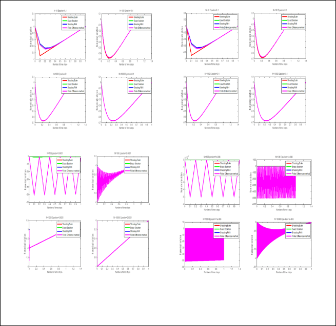
For a fixed 𝜖 the BVP of (3) in the boundary region [0,1] has
been solved. We observed in Figure.1 the Finite difference
method and the exact solution is equal that is invisible with eyes, also observed the shooting method using Euler method

IJSER © 2014 http://www.ijser.org

International Journal of Scientific & Engineering Research, Volume 5, Issue 5, May-2014 335

ISSN 2229-5518

are slightly far as well as using Runge-Kutta method from the exact solution are invisible to eyes because of the error rate are comparatively higher than Finite difference method
for 𝜖 = 1 with N=10 .We have investigated deeply insight in
Fig. 1 (a)&(b) the value of 𝜖 consider much more small as1
and 0.1 with increase of mesh size N the error rate with exact
solution as well as other numerical solution is quit low. In this situation numerical solution of shooting method and have not
been visible after that small value of 𝜖 the numerical
solution incapable of being seen and closely .In Fig.1(c) & (d)
we see that we have seen the waves running in step with just a small difference in amplitude and phase resulting from
small value of 𝜖 with the increases of N and the signal shown
as instability condition for numerical solution. In Finite
difference method, consider 𝜖 = 1 in Table II the error has
decreases with the increases of N where the order of accuracy
for finite difference method is the 2nd order for 𝜖 = 1& 0.1. We
have also seen in the Table.II has created much more and
more error for 𝜖 small. The error rate is high the stability of
finite difference method to create an oscillation becomes an
unstable as shown in Fig.1(d) an Figure.4.It can be seen from the numerical results presented in the previous section that the shooting method produces good approximation solution to BVP. It may be observed that the initial conditions assigned to new problems (derived from the original problem) are obtained easily from the solution of reduced problem.

8. CONCLUSION

We introduced the order of convergence of shooting and finite difference method for a general BVP. We have verify in Table I-II the theatrical analysis of the design and rate of
convergence is close to four for Runge-Kutta method and one for Euler method and also close to two for finite difference method. It’s shown minimum error for all methods for
damping coefficient 𝜖 = 1&0.1 and higher error for 𝜖 taken
smaller in this manner numerically diffused for both
methods.

REFERENCES

[1] Toro E.F., Riemann, “Solvers and Numerical methods for fluid dynamics”. Second edition, Springer 1999.

[2] A. A Slama,A.A.Mansour “Fourth-order Finite -differnce method for third-order boundary-value problem”Numerical Heat Transfer,Part B,47:383-401,2005.

[3] Lambert J D. Numerical methods for ordinary differential systems.

The initial value problem.John Wiley and Sons, 1997.

[4] Shampine L F, Gladwell I and Thompson S. Solving ODEs with

MATLAB. Cambridge University Press, 2003.

[5] Randall J. LeVeque “Finite Difference Methods for Differential Equations” AMath 585, Winter Quarter 2006 University of Washington Version of January, 2006.

[6] Zhilin Li, “Finite Difference Methods Basics” Center for Research in Scienti¯c Computation & Department of Mathematics North Carolina State University Raleigh, NC 27695.

[7] Bosho S. Jovanovic “Finite differenc schemes for boundary value

problems with gereralized solution” NOVI SAD J. MATH VOL.30,No.3,2000,45-58

[8] Riaz A Usmani “Finite difffernce methods for a certain two point

boundary value problem” Indian J. pure appl. Math., 14(3): 398-

411,March 1983.

[9] Raymond Hollsopple, Ram Venkataraman, David Doman “A modified Sipmle Shooting Method for Solving Two-Point Boundary- Value Problems”. IEEEAC paper # 1044, Vol. 6-2783

IJSER © 2014 http://www.ijser.org

International Journal of Scientific & Engineering Research, Volume 5, Issue 5, May-2014 336

ISSN 2229-5518

Table I. Computation results for Shooting method using Euler method and Fourth order Runge-Kutta
method for 𝜖 = 1,0.1, 10−4, 10−8.
Meth Nu

𝜖 = 1 𝜖 = 0.1 𝜖 = 10−4 𝜖 = 10−8
ods
mber of Mes
h size( N)
Error Order of
converge nce(p)
Error Order of
converge nce(p)
Error Order of
converge nce(p)
Err
or
Order of
converge nce(p)
Shoo
ting Meth od
Euler 10 0.0064
5739
100 0.0006
08022
1000 6.0447
2e-005
0.3678
51
1.02614 0.0191
896
1.00254 0.0018
4577
0 0
1.28261 0 NaN 0 NaN
1.01689 0 NaN 0 NaN
1000
6.0411
1.00025 0.0001
1.00164 0.3678
−∝ 0 NaN

Table II. Computation results for Finite difference method for ϵ=1, 0.1, 10-4, 10-8
Num

𝜖 = 1 𝜖 = 0.1 𝜖 = 10−4 𝜖 = 10−8
ber of
Error Order of
Error Order of
Error Order of
Error Order of

IJSER © 2014 http://www.ijser.org

International Journal of Scientific & Engineering Research, Volume 5, Issue 5, May-2014 337

ISSN 2229-5518

(a) (b)

(b) (d)

Fig.1. BVP for Finite difference method and Shooting method using Euler & 4th order Runge-Kutta method with

exact solution when (a) 𝜖 = 1 (b) 𝜖 = 0.1 (c) 𝜖 = 10−4 (d) 𝜖 = 108 and mesh size N=10, 100,1000,10000 with the

boundary value is a=0 and b=1.

IJSER © 2014 http://www.ijser.org