International Journal of Scientific & Engineering Research, Volume 5, Issue 5, May-2014 1351
ISSN 2229-5518
Review on Brain Tumor Detection Using Digital
Image Processing O. N. Pandey, Sandeep Panwar Jogi, Sarika Yadav, Veer Arjun, Vivek Kumar
Abstract— Medical image processing is the most challenging and emerging field today. This paper describes the methodology of detection & extraction of brain tumor from patient’s MRI scan images of the brain. In this paper, a method for segmentation of brain tumor has been developed on 2D-MRI data which allows the identification of tumor tissue with high accuracy and reproducibility compared to manual techniques.
This method incorporates with some noise removal functions, segmentation and morphological operations which are the basic concepts of image processing. Detection and extraction of tumor from MRI scan images of the brain is done by using MATLAB software. The aim of this work is to design an automated tool for brain tumor quantification using MRI image data sets.
Key words: Brain tumor, grey scale imaging, MRI, MATLAB, morphology, noise removal, segmentation.
—————————— ——————————
1 INTRODUCTION
Tumor is defined as the abnormal growth of the tissues [3]. Epilepsy is a brain disorder in which clusters of nerve cells, or neurons, in the brain sometimes signal abnormally [9]. Neurons normally generate electrochemical impulses that act on other neurons, glands, and muscles to produce human thoughts, feelings, and actions [6]. In epilepsy, the normal pattern of neuronal activity becomes disturbed, causing strange sensations, emotions, and behaviour or sometimes convulsions, muscle spasms, and loss of consciousness [20].
Magnetic Resonance Imaging (MRI) is an advanced medical imaging technique used to produce high quality images of the parts contained in the human body [12]. From these high- resolution images, we can derive detailed anatomical information to examine human brain development and discover abnormalities [30]. MRI consists of T1 weighted, T2 weighted and PD (proton density) weighted images and are processed by a system which integrates fuzzy based technique with multispectral analysis [1].
2 METHODOLOGY
The algorithm has two stages, first is pre-processing of given MRI image and after that segmentation and then morphological operations. Steps of algorithm are as following:-
1) Give MRI image of brain as input.
2) Convert it to gray scale image.
3) Apply high pass filter for noise removal.
4) Apply median filter to enhance the quality of image.
5) Compute threshold segmentation.
6) Compute watershed segmentation.
7) Compute morphological operation.

8) Finally output will be a tumor region.
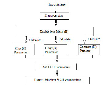
Figure 1. Proposed framework
2.1 The proposed framework
The process flow of our proposed methodology may be shown as figure 1.
The first section discusses how images are divided into regions using a block-based method. The second section shows how each classified block is studied individually by calculating its multiple parameter values. In this instance, the multiparameter features refer to the following three specific features: the edges (E), gray values (G), and local contrast (H) of the pixels in the block being analyzed [6].
IJSER © 2014 http://www.ijser.org
International Journal of Scientific & Engineering Research, Volume 5, Issue 5, May-2014 1352
ISSN 2229-5518
2.2 Input image
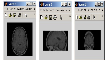
The images we got from MRI are of three types: axial Images, saggital Images, coronal Images. The number of images depends on the resolution of the movement of the MRI magnets [31].
E (r ,c ) =
∑
( x , y )∈B
( IEP == 1)
(3)
Preprocessing
In preprocessing the first step is to load the MRI image data set on to the MATLAB workspace and after loading they will be processed. After this processing there are only three clips instead of 384 separate images, i.e. one clip for axial images, one clip for saggital images and one clip for coronal images[6].
Axial, saggital and coronal images were loaded and viewed in the
MATLAB. After this, axial, saggital and coronal movie clips
Gray (G) Parameter: The gray parameter (G) for each block of the brain is accumulated, and controlled by a binary image (I T ) using the GD value as a threshold, as shown in equation (6). GD value is calculated using the average pixel value (Iavs ) of each image slice (S) for total image slices (T) of an image dataset, shown in equation (4) and (5).
were prepared and are shown in figure 2.
Iavs =

∑ p
65536
( x, y )
(4)

T

GD = ∑ Iavs
(5)
T S = 0
G (r ,c ) =
∑
( x , y )∈B
Ip ( x , y ), ∀ IT ( x , y ) = 1
(6)
Figure 2 Axial, saggital and coronal image chips
2.3 Multiparameter Calculations
Classifying regions using their multiparameter values makes the
Contrast (H) Parameter: Contrast (H) is often used to characterize the extent of variation in pixel intensity. We adopt the minimum/maximum stretch algorithm for the 8-neighborhood connectivity, where min H and max H represent the minimum and maximum intensity values of the neighbourhood pixel C8 (I H ), as shown in equation (7). In the previous studies, tumor cells are often associated with higher value of contrast (H) parameter (Senaratne et al., 2006). Hd is obtained by totaling the contrast of a supervised block, as shown in equation (8).
study of the regions of physiological and pathological interest
I ( )
I ( x , y ) − min H
× max H |H ∈ C ( I )
(7)
easier and more definable. The multiparameter features refer to the following three specific values for the edges (E), gray values (G), and local contrast (H) of the pixels [3].
H x , y

= 8 H
max H − min H
Edge (E) Parameter: We use sobel edge detection method to detect image edges (IE ) is obtained by filtering an input image with two convolution kernels concomitantly, one to detect
Hd (r ,c ) =
∑ H
( x , y )∈B
( x , y )
(8)
changes in vertical contrast (HX ) and the other to detect horizontal contrast (HY ), shown in equation (1). Image output (I E ) is obtained by calculating the gradient magnitude of each pixel, as shown in equation (2). Subsequently, the edge parameter (E) is calculated, whereby E (r,c) is increased by one each time when IE (x, y) = ‘1’ in a supervised block, as shown in equation (3). [24]
2.4 Segmentation of brain tumor using Region of Interest
(ROI) Command
As it has been seen from the above result that high density images have been separated from the MRI images using watershed
segmentation. Here main aim is to segment the tumor from the
−1 0 1
−1 −2
−1
MRI images. This can be done by using the ROI command in
MATLAB. After the application of the ROI command, the tumor
HX = −2 0 2 , HY = 0 0 0
(1)
−1 0 1
1 2 1
may be segmented. This can be achieved by executing the
algorithm in MATLAB[4].

I ( x, y ) =
I ( x, y ) + I ( x, y )
(2)
All the calculations and techniques can be summarized in
E x Y
following steps for the tumor detection:
I. Greyscale Imaging: MRI images are magnetic resonance scan of a patient taken with the help of a computer. Generally a greyscale looks like black
IJSER © 2014 http://www.ijser.org
International Journal of Scientific & Engineering Research, Volume 5, Issue 5, May-2014 1353
ISSN 2229-5518
and white images [25]. The illusion of gray shading in a halftone image is obtained by rendering the
image as a grid of black dots on a white background (or vice-versa), with sizes of individual dots determining the apparent lightness of the gray in their vicinity. In the case of transmitted light (for example, the image on a computer display), the brightness levels of the red (R), green (G) and blue (B) components are each represented as a number from decimal 0 to 255, or binary 00000000 to
11111111. For every pixel in a red-green-blue
(RGB ) greyscale image, R = G = B. The lightness of the gray is directly proportional to the number representing the brightness levels of the primary colours. Black is represented by R = G = B = 0 or R
= G = B = 00000000, and white is represented by R
= G = B = 255 or R = G = B = 11111111. Because
there are 8 bits in the binary representation of the gray level, this imaging method is called 8-bit greyscale [18].
The darkest possible shade is black, which is the
total absence of transmitted or reflected light. The lightest possible shade is white, the total transmission or reflection of light at all visible wavelengths. So because of the above reason first we convert our MRI image to be pre-processed in greyscale image [1].
II. High Pass Filter: A high pass filter is method for sharpening methods. An image is sharpened when contrast is enhanced between adjoining areas with variation in brightness or darkness. The kernel array of the high pass filter is designed to increase the brightness of the centre pixel relative to neighbouring pixels. The kernel array contains a positive value surrounded by negative values [8].
III. Medial filter: Median filter is very widely used in digital image processing because, under certain conditions, it preserves edge while removing noise. [13] The task of filtering is performed by the median filter by use of window that is a pattern of neighbours. The window pattern slides, entry by entry, over the entire signals. The middle value of the window is decided by the median value of all the entries at a time.
IV. Threshold segmentation: This method is based on clip-level (or threshold value) to turn a gray-scale image into a binary image by selecting a threshold value. Segmentation is the process of partitioning a digital image into multiple segments, called superpixels. [18] Image segmentation is typically used to locate objects and boundaries in images. By thresholding we assign a specific level to each pixel in image according to the similarity in visual characteristics [5].
V. Watershed segmentation: A grey-scale may be seen as a topographic relief, where the grey level of a pixel is interpreted as its altitude in the relief. In
image processing, different watershed lines may be computed. Mayor’s flooding Watershed algorithm is used to compute the watershed segmentation [14]. This algorithm works on a grey scale image. During the successive flooding of the grey value relief, watersheds with adjacent catchment basins are constructed. This flooding process is performed on the gradient image, i.e. the basins should emerge along the edges. Normally this will lead to an over- segmentation of the image, especially for noisy image material, e.g. medical CT data. Either the image must be preprocessed or the regions must be merged on the basis of a similarity criterion afterwards. [28]
VI. Morphological Operations: Morphological operation is defined as the relative ordering of all the pixel values, not on their numerical values, and therefore are especially suited for the processing of binary images. Morphological techniques probe an image with a small shape or template called a structuring element. The structuring element is positioned at all possible locations in the image and it is compared with the corresponding neighbourhood of pixels. Some operations test whether the element "fits" within the neighbourhood, while others test whether it "hits" or intersects the neighbourhood.
A morphological operation on a binary image creates a new binary image in which the pixel has a non-zero value only if the test is successful at that location in the input image. [31]
3 RESULT AND CONCLUSSION
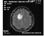
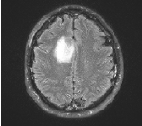
The discussed methodology can be made clearer by considering an MRI image of tumor affected brain, shown in figure 3, and then performing all the operations in a sequence.

Figure 3 MRI image of tumor affected brain
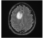
We get greyscale image of the MRI image as shown in figure 4.
IJSER © 2014 http://www.ijser.org
International Journal of Scientific & Engineering Research, Volume 5, Issue 5, May-2014 1354
ISSN 2229-5518

Figure 4 Greyscale image
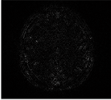
On performing high pass filtering on the greyscale image of figure 4 the HPF output is obtained as shown in figure 5.

Figure 5 HPF output
There may be some noise in the greyscale image of the brain, agter removing the noise the enhanced MRI image is figure 6.

Figure 6 Enhanced MRI image
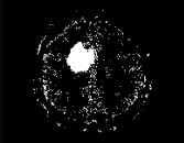
The MRI greyscale image is converted into a binary image by applying threshold segmentation and given in figure 7 [18].

Figure 7 Threshold segmented image of input image
For more accurate and precise result, watershed segmentation is done on the threshold segmented image and we get the output
image as shown in figure 8.

Figure 8 Watershed segmented image of input image
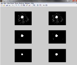
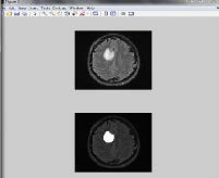
After the watershed segmentation the relative ordering of the pixel value of the image is done by morphological operation and the output in each step is shown in figure 9.

Figure 9 Morphological operations
Finally, on observing the difference in brightness or darkness in the MRI image, the brain tumor can be detected as given in figure
10.

Figure 10 Final Extracted brain tumor from MRI image
4 FUTURE DIRECTION
IJSER © 2014 http://www.ijser.org
International Journal of Scientific & Engineering Research, Volume 5, Issue 5, May-2014 1355
ISSN 2229-5518
In future this programme can be done more advanced so that major tumor can be classified according to its type [16].
Advancement in programming can help the segmentation completely automatic. By plotting the graph the growth of the tumor can be analysed [9].
REFERENCES
[1]. W. Gonzalez, “Digital Image Processing”, 2nd ed. Prentice
Hall, Year of Publication 2008, Page no 378.
[2]. S. Murugavalli, V. Rajamani, “A high speed parallel fuzzy c-
mean algorithm for brain tumor segmentation”,” BIME Journal”, Vol. no:06, Issue (1), Dec., 2006
[3]. Mohamed Lamine Toure, “Advanced Algorithm for Brain Segmentation using Fuzzy to Localize Cancer and Epilepsy Region”, International Conference on Electronics and Information Engineering (ICEIE 2010), Vol. no 2 .
[4]. Dr.G.Padmavathi, Mr.M.Muthukumar and Mr. Suresh Kumar Thakur, “Non linear Image segmentation using fuzzy c means clustering method with thresholding for underwater images”, IJCSI International Journal of Computer Science Issues, Vol. 7, Issue 3, No 9, May 2010
[5]. Matei Mancas, Bernard Gosselin, Benoît macq, “Segmentation Using a Region Growing Thresholding”
[6]. T .Logeswari and M.Karnan “An improved implementation of brain tumor detection using segmentation based on soft computing” Journal of Cancer Research and Experimental Oncology Vol. 2(1) pp. 006-014, March, 2010
[7]. Wankai Deng , Wei Xiao, Chao Pan, Jianguo Liu Key “MRI brain tumor segmentation based on improved fuzzy c-means” Method. Laboratory of Education Ministry for Image Processing and Intelligence Control Institute for Pattern Recognition and Artificial Intelligence SPIE Vol. 7497, 74972N, 2009
[8]. Abbasi S and Mokhtarian F (2001) Affine-similar shape
retrieval: application to multiview 3-D object recognition. IEEE Trans. Image processing. 10 (1), 31-139.
[9]. Abdel-Halim Elamy and Maidong Hu (2007) Mining brain tumors & their growth rates. IEEE Image Processing Society Journal. pp: 872-875.
[10]. Bailet JW, Alan Lichtenstein, Ge Chen and Robert A.
Mickel (1997) Inhibition of lymphocyte function by head and neck carcinoma cell line soluble factors. Arch Otolaryngol Head Neck Surg.123(8),855-862.
[11]. Bailet JW, Abemayor E, Jabour BA, Hawkins RA, Hoh CK
and Ward PH (1992) Positron emission tomogarphy: a new precise modality for detection of primary head and neck tumor and assessment of cervical adenopathy. Laryngosope. 102, 281-
288.
[12]. Black PM, Moriarty T and Alexander E (1997) Development and implementation of intraoperative magnetic resonance imaging and its neurosurgical applications. Neurosurgery. 41(4), 831-845.
[13]. Bountris P, Farantatos E and Apostolou N (2005) Advanced image analysis tool development for the early stage bronchial cancer detection. PWASET. 9, 151-156.
[14]. Deng Y, Manjunath BS, Kenney C, Moore MS and Shin H (2001) An efficient color representation for image retrieval. IEEE Trans. Image Processing. 10 (1), 140-147.
[15]. Dewalle Vignion AS, Betrouni N and Makni N (2008) A
new method based on both fuzzy set and possibility theories for
tumor volume segmentation on PET images. 30th Annual
International IEEE EMBS Conference. 3122-3125.
[16]. Epifano I and Ayala G (2002) A random set view of texture classification. IEEE Trans. Image Processing. 11(8), 859-867. [17]. Fadi Abu Amara and Abdel Qadar (2007) Detection of breast cancer using independent component analysis. IEEE EIT Proceedings. 236- 241.
[18]. Gering D, Eric W, Grimson L and Kikinis R (2002) Recognizing deviations from normalcy for brain tumor segmentation. Medical Image Computing and Computer-Assisted Intervention (MICCAI), Tokyo Japan.pp:388-395 (http://link.springer./link/service/series/0558/bibs/2488/24880388
.htm).
[19]. Gupta R and Undril P (1995) The use of textureanalysis to delineate suspicious masses in mammograohy. Physics in Medicine & Biology. 40,835-855.
[20]. Haney SM, Thompson PM, Cloughesy TF, Alger JR and
Toga AW (2001) Tracking tumor growth rates in patients with malignant gliomas: a test of two algorithms. AJNR Am. J. Neuroradiology. 22,73-82.
[21]. Hinz M, Pohle R, Shin H and Tonnies KD (2002) Region-
based interactive 3D image analysis of structures in medical data by hybrid rendering. Proc. SPIE in Visualization, Image-Guided Procedures, and Display. 4681, 388-395.
[22]. Jason J. Corso, Eitan Sharon and Shishir Dube (2008)
Efficient Multilevel Brain Tumor Segmentation with Integrated Bayesian Model Classification. IEEE Transaction on Medical Imaging. 27, 148-155.
[23]. Jolesz FA (1997) Image-guided procedures and the
operating room of the future. Radiology. 204,601-612.
[24]. Krishnan K and Atkins MS (1998) Segmentation of multiple
sclerosis lesions in MRI – an image analysis approach. Proc of the
SPIE Medical Imaging. 338, 1106-1116.
[25]. Lihua Li, Weidong Xu, Zuobao Wu, Angela Salem and Claudia Berman (2007) A new computerized method for missed cancer detection in screening mammography. Proc. IEEE Natnl. Conf. on Integration Technol. pp: 21-25.
[26]. Nacim Betrouni, Phillipe Puech and Anne Sophie Dewalle
(2007) 3 D automatic segmentation and reconstruction of prostate on MRI images. Proc. 29th Annual Intnl. Conf. IEEE EMBS.
5259-5262.
[27]. Nakajima S, Atsumi H and Bhalerao AH (1997) Computer-
assisted surgical planning for cerebrovascular neurosurgery. Neurosurgery. 41, 403-409.
[28]. Radu Calinescu and Steve Harris (2007) Model driven architecture for cancer research. IEEE Intnl. Conf. Software Engg. Formal Methods. pp: 59-68.
[29]. Senaratne GG, Richard B. Keam, Winston L. Sweatman and
Greame C. Wake (2006) Solution to the 2 dimensional boundary value problem for microwave breast tumor detection. IEEE Microwave & Wireless Component Letters. 16(10), 343-348.
[30]. Vailaya S, Figueriodo MAT, Jain AK, and Zhang HJ (2001)
Image classification for content-based Indering. IEEE Trans. Image processing. 10(1), 117-130.
[31]. Yao Yao (2004) Segmentation of breast cancer mass in mammograms and detection using Magnetic Resonance Imaging. IEEE Image Processing Soc. J. pp: 561-567.
IJSER © 2014 http://www.ijser.org
