The research paper published by IJSER journal is about Rainfall analysis and design flood estimation for Upper Krishna River Basin Catchment in India 1

ISSN 2229-5518

Rainfall analysis and design flood estimation for

Upper Krishna River Basin Catchment in India

B.K.Sathe, M.V.Khir, R.N. Sankhua

Abstracts

Design flood estimates have been carried out for Upper Krishna basin catchment employing flood frequency analysis methods for planning and or infrastructure design. This method consists of fitting a theoretical extreme-value probability distribution to the maximum annual flow rate data collected at a stream flow gauging station, thus enabling the hydrologist to estimate, via extrapolation, the flow rate or peak discharge corresponding to a given design return period. Seven gauging sites were analyz ed with a view to predicting the floods of different return periods. Flood frequency analysis is carried out by Gumble’s distribution. Detail rainfall analysis also done with river cross sections. High flood levels are mark on the river cross sections which he lps for design of hydraulic structures like bridges, culverts etc. The results of the investigation are analyzed and discussed and useful conclusions are drawn.

Keywords : Gumbel distribution; Flood frequency ;Design flood;

INTRODUCTION

The estimation of peak flow of a design return period is a necessary task in many civil engineering projects such as those involving design of bridge openings and culverts, drainage networks, flood relief/protection schemes, the assessment of flood risk and the determination of the ‗finish-floor level‘ for
both commercial and large-scale residential
developments.(Bedient P.B.(1987))
Flood estimates are also required for the safe operation of flood control structures, for taking emergency measures such as maintenance of flood levees, evacuating the people to safe localities etc. Floods not only damage properties and endanger the lives of humans and animals, but also have negative effects on the environment and aquatic life. These include soil erosion,
sediment deposition downstream and destruction of spawning

IJSER © 2012 http://www.ijser.org

The research paper published by IJSER journal is about Rainfall analysis and design flood estimation for Upper Krishna River Basin Catchment in India 2

ISSN 2229-5518

grounds for fish and other wildlife habitat. The analysis of flood
frequency of river catchment has therefore become imperative in
order to curtail hazards of this nature. Flood frequency analysis involves using observed annual peak flow discharge data to compute statistical information such as mean values, standard deviation, skewness and recurrence interval of flood.These statistical data are then used to construct frequency distributions, which are graphs and tables that tell the likelihood of various discharges as a function of recurrence interval or exceedance probability. (BaylissA.C.1999b) Flood frequency distribution can take many forms depending on the equations used to carry out the statistical analysis.
In the design of practically all hydrologic structures the peak flow that can be expected with an assigned frequency (say 1 in
100 years) is of primary importance to adequately design the
structure to accommodate its effect. The design of bridges, culvert waterways and spillways for dams and estimation of scour at a hydraulic structure are some examples wherein flood- peak values are required. To estimate the magnitude of a flood peak the following methods are available:

Research Scholar, CSRE, IIT-Bombay

Associate Professor, CSRE, IIT-Bombay

Director ,National Water Academy,Pune

Corresponding author: bksathe@yahoo.co.in
1. Rational method,
2. Empirical method,
3. Unit-hydrograph technique, and
4. Flood-frequency studies.
The use of a particular method depends upon (i) the desired objective, (ii) the available data and (iii) the importance of the project. Further, the rational method is applicable only to small- size (<50 km2) catchments and the unit-hydrograph method is normally restricted to moderate-size catchments with areas less than 5000 km2.(Bhattari K.P.,2004)The main focus of this paper is on flood frequency analysis of hydrological data is to determine relationship of peak discharge - return period at any site on a river so as to obtain a useful estimate of design flood of extreme event for a selected return period.
Floods are exceedingly complex natural events consisting of a number of component parameters of the hydrologic system and very difficult to model analytically. There are two broad categories of research in flood frequency analysis, namely,
‗regionalization‘ and ‗at-site‘. Regionalization research investigates the relationship between flood frequency curves of catchments at different locations whereas at-site research investigates the relationship between peak flood discharge and its frequency of occurrence for a single catchment.(Dalrymple T.(1960)) Before carrying out flood frequency analysis of a given flood data series, the hydrologist has to decide on the following
three options:

IJSER © 2012 http://www.ijser.org

The research paper published by IJSER journal is about Rainfall analysis and design flood estimation for Upper Krishna River Basin Catchment in India 3

ISSN 2229-5518

Selection of a suitable flood frequency model (e.g. annual maxim series model, partial duration series or peak over threshold model, or time series model)
Selection of a suitable statistical distribution (e.g. Generalized
Extreme Value Distribution, Exponential Distribution, General
Logistic Distribution)
Selection of a parameter estimation method to fit the selected distribution to the given flood data, (e.g. the method of ordinary moments, probability weighted moments, L-moments etc.) Another approach to the prediction of flood flows, and also applicable to other hydrologic process such as rainfall etc. is the
statistical method of frequency analysis.(Chow V.T.(1964))
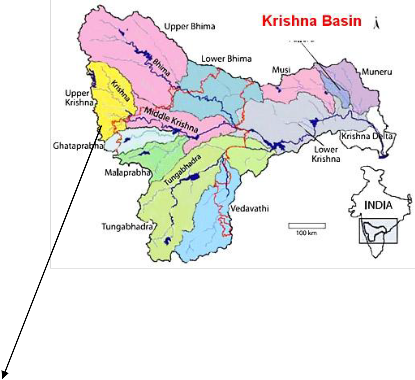
The study area comprises of an upland watershed and a major tributary of Krishna River in the upper Krishna basin. The river has its source in the Western Ghats on the leeward side of the mountains Maharashtra, India. The river is 310 kms long and the catchment covers an area of 14,539 sq. km falling in Survey of India (SOI) toposheet No: 47 /K,47 /L,47 / P on 1:250,000 scale. The investigated area is enclosed between latitudes 17°18‘N and
16°15′N and longitudes 73°50′E and 75°54′E. (Figure 1)

DATA USED

The annual peak flood series data for 10 years varying over period 1965 to 2010 for 7 important stations such as Karad
,Warna, Arjunwad, Kurundwad, Warungi of Upper Krishna

THE STUDY AREA

TABLE-1

basin. The data were collected from the Maharashtra state
irrigation department.(Table 1) (Table 5)

GAUGING STATIONS IN STUDY AREA

METHODOLOGY

Before the analysis, the hydrological data were selected to fairly
satisfy the assumptions of independence and identical
distribution. This is achieved by selecting the annual maximum

IJSER © 2012 http://www.ijser.org

The research paper published by IJSER journal is about Rainfall analysis and design flood estimation for Upper Krishna River Basin Catchment in India 4

ISSN 2229-5518

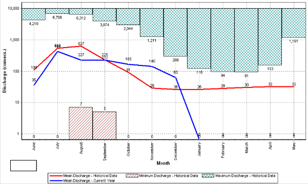
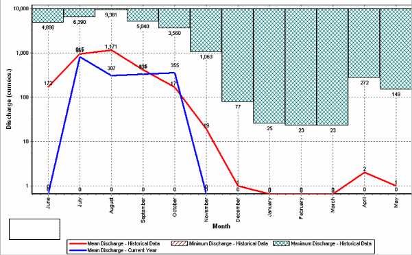
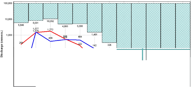
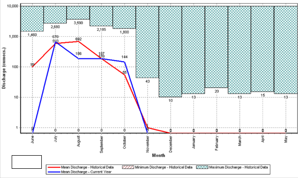
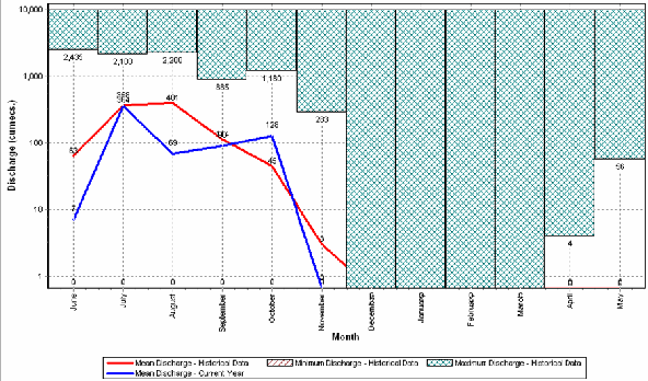
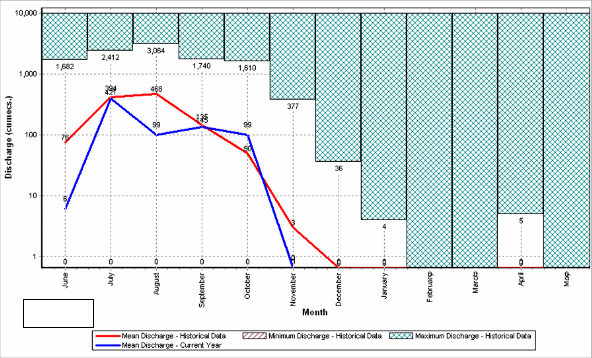
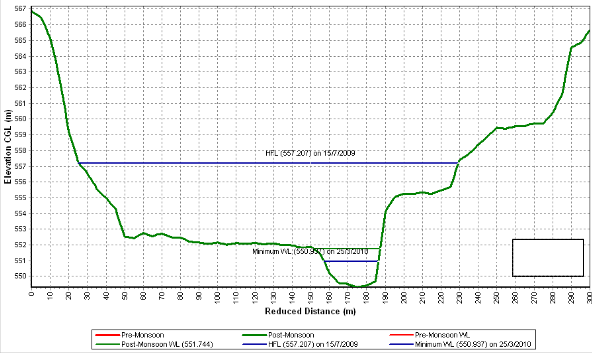
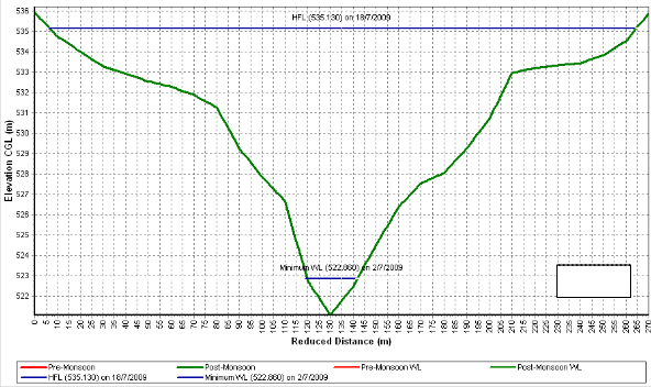
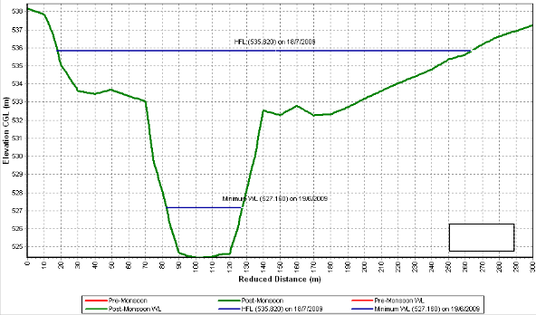
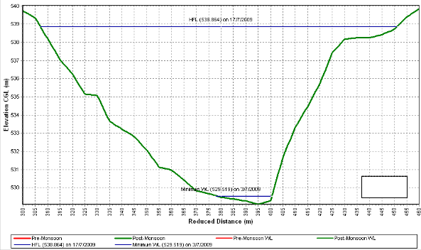
of the variable being analyzed, which may be the largest instantaneous peak flow occurring at any time during the year (Figure 3).For instantaneous peak flow for all seven gauging stations, mean highest dishcharge,minimum discharge for the year 1965 to 2010 are analyzed statistically and graphs are plot as rainfall analysis, hydraulic data of river cross section and observed high flood levels (HFL) for pre monsoon and post monsoon are analyzed to estimate peak flow and high flood levels marks which required to design of bridge opening,culverts,drainage networks.(Figure 4) .The discharge analyzed was assumed to be independent and identically distributed, and the hydrological system producing them considered being stochastic, space and time independent. (Stediner J.R. and Tasker G.D. (1986)).

3.1 PROBABILITY OF FLOOD OCCURRENCE

The return period is said to be the average interval in years between occurrence of a flood of specific magnitude and an equal or larger flood. The m th largest flood in a data series has been equaled or exceeded m times in the period of record N years and an estimate of its recurrence interval, TP,(eqn3) (Table
3) as given by Weibull formula (Dalrymple T.(1960))
P = m / n +1, eqn… (1)
where, P is the probability of the event. ‗m‘ is the rank and ‗n‘ is the number of data points (years of data).
Since the only possibilities are that the event will or will not
occur in any year, the probability that it will not occur in a given
year is 1 –P. From the principles of probability, the probability J that at least one event that equals or exceeds the T year event will occur in any series of N years is:
J = 1 – (1 – P) N eqn…(2)
Hence, J = 1 – (1 –T) N is the probability that the event will occur during a span of N years (Linsley and Frazini, 1992).The values of the annual maximum flood from a given catchment area for large number of successive years constitute a hydrologic data series called the annual series. The data are then arranged in decreasing order of magnitude and the probability P of each event being equaled to or exceeded (plotting position) is calculated by the plotting-position formula (eqn… 1)
Where, m = order number of the event and N = total number of
events in the data. The recurrence interval, Tp ( also called the return period or frequency ) is calculated as
Tp = 1 / P eqn…(3)
A plot of discharge Q vs. Tp yields the probability distribution. For small return periods (i.e. for interpolation) or where limited extrapolation is required, a simple best-fitting curve through plotted points can be used as the probability distribution. A logarithmic scale for Tp is often advantageous. However, when larger extrapolations of Tp are involved, theoretical probability distribution have to be used. In frequency analysis of floods the usual problem is to predict extreme flood events. Towards this, specific extreme-value distributions are assumed and the required statistical parameters calculated from the available data. Using these, the flood magnitude for a specific period is
estimated. Chow (1951) has shown that most frequency-

IJSER © 2012 http://www.ijser.org

The research paper published by IJSER journal is about Rainfall analysis and design flood estimation for Upper Krishna River Basin Catchment in India 5

ISSN 2229-5518

distribution functions applicable in hydraulic studies can be expressed by the following equation known as the general equation of hydrologic frequency analysis:
X= x +Kσ eqn ….(4)
Where, X = value of the variant; Q of a random hydrologic series with a return period Tp;
x = mean of the variants; σ = standard deviation of the variant; K
= frequency factor which depends upon the return period; Tp and the assumed frequency distribution. Some of the commonly used frequency distribution functions for the prediction of extreme flood values are:
Gumbel‘s extreme-value distribution, Log-Pearson Type III
distribution, and Log normal distribution.
Only the Gumbel distribution is dealt here with emphasis on application.

3.2 GUMBEL’S METHOD

Gumbel defined a flood as the largest of the 365 daily flows and the annual series of flood flows constitute a series of largest values of flows. According to his theory of extreme events, the probability of occurrence of an event equal to or larger than a value xo is

P ( ) = 1- eqn…(5)

In which y is a dimensionless variable given by

y = α ( x – a )

a = x – 0.45005 σx eqn…(6)

α = 1.2825 / σx

Thus, y = (1.2825(x - x) / σx) + 0.577

Where x = mean and σx = standard deviation of the variant X.
In practice it is the value of X
for a given P that is required and as such Eq. (5) is transposed as

yp = - ln [ - ln ( 1 – P )] eqn…(7)

Noting that the return period Tp = 1/P and designating

yT = The value of y, commonly called the reduced variate, for a given

yT = - [ln.ln.(Tp/(Tp-1))] eqn… (7.1)

or
yT = - [0.834 + 2.303 log.log.(Tp/(Tp-1))] .. eqn…(7.2)
Now rearranging Eq. (5), the value of the variants X with a return period Tp is

XT = x + Kσ x eqn…(8)

X T is estimated event magnitude

Where K = (yT – 0.577)/1.2825 eqn…(9)

Note that eqn (9) is of the same form as the general equation of hydrologic frequency analysis, Eq. (4). Further eqns. (8) and (9) constitute the basic Gumbel‘s equations and are applicable to an
infinite sample size (i.e. N→∝ ).Since practical annual data series
of extreme events such as floods, maximum rainfall depths, etc.,
all have finite lengths of record, eqn (9) is modified to account for finite N as given below for practical use.

3.2.1 GUMBEL’S EQUATION FOR PRACTICAL USE Equation (8) giving the values of the variate X with a recurrence interval Tp is used as

XT= x+K σ n-1 eqn… (10)

Where σ n-1= standard deviation of the sample size N

K= frequency factor expressed as

IJSER © 2012 http://www.ijser.org

The research paper published by IJSER journal is about Rainfall analysis and design flood estimation for Upper Krishna River Basin Catchment in India 6

ISSN 2229-5518

K = ( yT – yn /Sn ) eqn…(11)

In which yT = reduced variate, a function of T and is given by

y = - [ln.ln.(Tp/(Tp-1))] eqn… (12)

or

yT = -[0.834 + 2.303 log.log.(Tp/(Tp-1))]

yn = reduced mean, a function of sample size N

Sn = reduced standard deviation, a function of sample size N These equations are using the following procedure to estimate

the flood magnitude corresponding to a given return period based on an annual flood series.
1. The discharge data are compiled with the sample size N (Table 5). Here, the annual flood value is the variate X. For the
given data, x and σn-1 values are found. Using standard tables
(Table 2) yn and Sn appropriate to given N are determined For a given T, K and yT are found by using eq. (11 and 12) and required xT is determined by eq. (10).
To verify whether the given data follow the assumed Gumbel‘s
distribution, the following procedure was adopted.
The value of XT for some return periods Tp < N are calculated by using Gumbel‘s formula and plotted as XT vs Tp on a convenient paper such as a semi-log, log-log or Gumbel

probability paper (Figure-2). The use of Gumbel probability paper results in a straight line for XT vsTp plot. Gumble‘s distribution has the property which gives

Tp = 2.33years for the average of the annual series when N is very large. Thus, the value of a flood with Tp = 2.33 years is
called the mean annual flood. In graphical plots this gives a
mandatory point through which the line showing variation of XT with Tp must pass. For the given data, values of return periods (plotting positions) for various recorded values, x of the variate are obtained by the relation

Tp= ( N+1)/m and plotted on the graph described above. A

good fit of observed data with the theoretical variation line indicates the applicability of Gumbel‘s distribution to the given data series by extrapolation of the straight line XT vs Tp,values

of XT for Tp> N can be determined easily.

4. FLOOD DISCHARGE COMPUTATION AND ANALYSIS

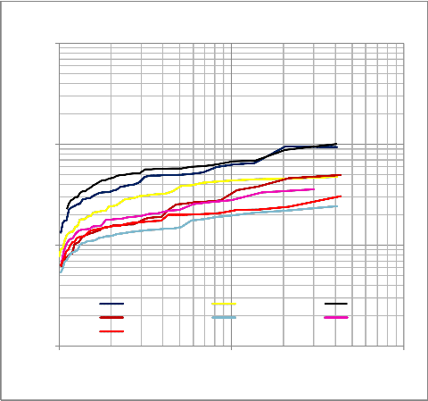
The flood discharge values are arranged in descending order and the plotting position recurrence interval Tp for each discharge is obtained as

Tp = (N + 1) / m = 41 / m

Where m = order number. The discharge magnitude Q are plotted against the corresponding to Tp on a Gumbel extreme probability paper (Figure- 2).The statistics x and σn-1 for the
series are next calculated and are shown in Table 2.Using these
the discharge XT for some chosen recurrence interval is calculated by using Gumbel‘s formulae [Eqs. (12), (11) and (10)].From the standard tables of Gumbel‘s extreme value
distribution, for N = 40, yn =0.5436
and Sn = 1.1413.Choosing Tp = 50 years, by eqn. (12)

yT = -[ln.ln(50/ 49)] = 2.056, K = (2.056 -0.5485) /1.607 =

0.938

XT = 3536.222+ (0.938 x1813.04) = 5236.8535 m3/s

IJSER © 2012 http://www.ijser.org

The research paper published by IJSER journal is about Rainfall analysis and design flood estimation for Upper Krishna River Basin Catchment in India 7

ISSN 2229-5518

TABLE -2:

REDUCED MEAN (YN ) AND REDUCED STANDARD DEVIATION ( SN)

TABLE-3

TP FOR OBSERVED DATA FOR ARJUNWAD GAUGE STATION

Order
Number M
Flood Discharge
(m3 / s)
Tp Order Number
M

IJSER © 2012 http://www.ijser.org

Flood Discharge Tp
(m3 / s)

The research paper published by IJSER journal is about Rainfall analysis and design flood estimation for Upper Krishna River Basin Catchment in India 8

ISSN 2229-5518

N = 40 years, x = 3536.22 m3 / s, σ n-1 = 1813.04m3 /s
Similarly , values of XT are calculated for more Tp values

TABLE-4:

DESIGN DISCHARGE FOR RETURN PERIOD TP

Tp Design discharge XT ( obtained by eq.10 )

TABLE 5:

ANNUAL MAXIMUM DISCHARGE W ITH CORRESPONDING WATER LEVEL (M.S.L.) FOR ARJUNWAD

IJSER © 2012 http://www.ijser.org

The research paper published by IJSER journal is about Rainfall analysis and design flood estimation for Upper Krishna River Basin Catchment in India 9

ISSN 2229-5518

a

CONCLUSIONS

In the present study of flood frequency analysis, annual maximum series data pertaining to period 1962-2010 for the Karad, Sangli, Kholapur were analyzed using Gumble‘s distribution method for 2,10,20,50 100,200 year return period
flood for each gauging station. The design storm rainfall of
various return periods have been computed from statistical analysis of point and areal time series annual maximum discharge. It has been observed that design floods for return period of 2 year were flood to be almost same as the observed data and verified with historical data. Arjunwad river gauging
station is having very high design flood as compare to other

IJSER © 2012 http://www.ijser.org

The research paper published by IJSER journal is about Rainfall analysis and design flood estimation for Upper Krishna River Basin Catchment in India 10

ISSN 2229-5518

gauging station in the study area. The method of plotting annual flood peaks and fitting a Gumble distribution is valid for any year period chosen. Application of Gumble‘s distribution indicates a very good fit of observed data series with theoretical
variation. The main finding of this study are the 1 in 100 year
return period recommended for design of river control works is
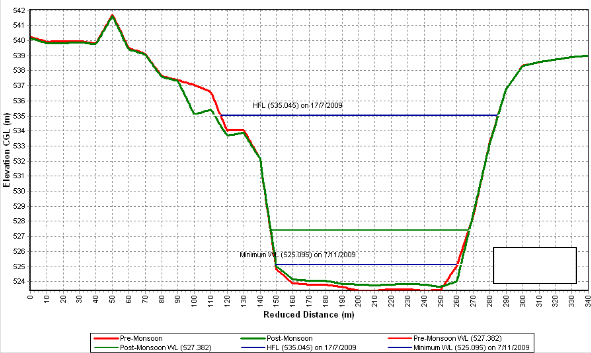
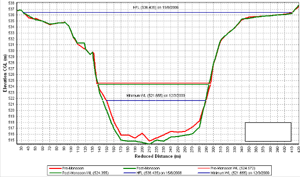
6,246 m3/s. Knowing these design floods one can mark the high flood water level with the help of available river cross sectional area and can be used in flood studies and design of hydraulic structures within the basin and similar catchments.

IJSER © 2012 http://www.ijser.org

The research paper published by IJSER journal is about Rainfall analysis and design flood estimation for Upper Krishna River Basin Catchment in India 11

ISSN 2229-5518

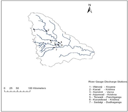
Figure 1 : Study Area

Figure.2: Flood probability analysis by Gumble’s distribution

IJSER © 2012 http://www.ijser.org

The research paper published by IJSER journal is about Rainfall analysis and design flood estimation for Upper Krishna River Basin Catchment in India 12

ISSN 2229-5518

100000

Recurrence Interval Plot -

10000

1000

100

Arjunwad Karad Kurundwad Warungi Sadalgi Terwad Samdoli

1.00 10.00 100.00

Recurrence Interval (years) (TP = N+1 / m )

Figure 3: Time – Discharge analysis for year 2009 -10 for all seven Gauging stations

IJSER © 2012 http://www.ijser.org

The research paper published by IJSER journal is about Rainfall analysis and design flood estimation for Upper Krishna River Basin Catchment in India 13

ISSN 2229-5518

Karad

Arjunwad

IJSER © 2012 http://www.ijser.org

Internatio nal Jo urnal of Scientif ic & Engineering Resea rch Volume 3, Issue 8, A ugust-2012 14

ISSN 2229-5518

-1-0-0---------

10

···r.··········-.'···········r'-·······--·.,'···

42 >QQ<XXX; 47 48

27

.......'....................................'............'...............................................................................

I I I I I I

0 0 0 0 0

j

... ...

...

... ... I i i e !

II!

i :":E

Kurundwad

ti

l 0 z

k!

0

Month

...

....

::E

Mean Oisolwge - HistoricalD$1a IZZZZJ Minimum Discharge - HistoricalD$1a Maximum Discharge - Historical D$1a

- Mean DiSCher e- Current Vear

r..i

5

..

4W3 4,641 «

2, 00 2,75

-----:-----------!-----------:-----------!········1-·-,- «

530

1:'

"...,

Q"'

: I :

' . ' : : : IS

' '

il ;is

--- --!-----------!--- ------+---------!-----------!----------f-------:- --········!··---------!-----------!········--·l·-·········!··-··

I I I I 0 I 0 I I I

0 I I I 0 0 I 0 I I

0 I I I I I I I I I I I I I 0 I I I I I I 0 I I 0 0 0 I 0 0

····?·I ··········?·0 --------?···········?·········?·····I ·· .------I --------------0-- ----------0---------

I t I 0

i J t ! t I i I i i

00 0 z 0 -

waruji Month

-- lllean Discharge • Historical Data I1ZZZJMnrum Discharge - Historical Data Maxnun Discharge - Historical Data

-- Mean Dischar -Current Yet11

IJSER lb)2012 http://www ijser orq

The research paper published by IJSER journal is about Rainfall analysis and design flood estimation for Upper Krishna River Basin Catchment in India 15

ISSN 2229-5518

Terwa

IJSER © 2012 http://www.ijser.org

The research paper published by IJSER journal is about Rainfall analysis and design flood estimation for Upper Krishna River Basin Catchment in India 16

ISSN 2229-5518

samdoli

Figure 4 River cross section with high flood levels for river gauging station

Kara

IJSER © 2012 http://www.ijser.org

The research paper published by IJSER journal is about Rainfall analysis and design flood estimation for Upper Krishna River Basin Catchment in India 17

ISSN 2229-5518

Arjunwad

Kurundwad

IJSER © 2012 http://www.ijser.org

The research paper published by IJSER journal is about Rainfall analysis and design flood estimation for Upper Krishna River Basin Catchment in India 18

ISSN 2229-5518

Warunji

Terwad

IJSER © 2012 http://www.ijser.org

The research paper published by IJSER journal is about Rainfall analysis and design flood estimation for Upper Krishna River Basin Catchment in India 19

ISSN 2229-5518

Sadalgi

Samdol

REFERENCES

[1] A.K.Kulkarni (1994) ‗A study of heavy rainfall 22-23 August, 1990 over

Vidarbha region of Maharashtra.‘Trans.Inst.Indian

Geographers.Vol.16.No.11994

[2] Adamwonski K (1985). Non parametric Kernel estimate of flood frequency,

IJSER © 2012 http://www.ijser.org

The research paper published by IJSER journal is about Rainfall analysis and design flood estimation for Upper Krishna River Basin Catchment in India 20

ISSN 2229-5518

Water resources, pp-1585-90.

[3] Analysis Techniques: (2005), ‗Flood Frequency Analysis Tutorial with Instantaneous Peak Data fromStreamflow Evaluations for Watershed Restoration Planning and Design,‘ http://water.oregonstate.edu/streamflow/, Oregon State University

[4] Bayliss, A.C. (1999b). Catchment descriptors. Vol. 5, Flood Estimation

Handbook. Institute of Hydrology, Wallingford, pp-130

[5] Bedient P. B. (1987). Hydrology and flood plain analysis. Wesley. 12056, pp.

165 - 179.

[6] Bhattarai, K. P. (1997) Use of L-moments in flood frequency analysis. MSc

Thesis, National University of Ireland, Galway.

[7] Bhattarai, K.P. (2004). Partial L-moments for the analysis of censored flood samples. Journal of Hydrological Sciences, Vol. 49 (5), pp-855-868.

[8] Central Water and Power Commission (1969), Estimation of Design Flood-

Recommended Procedure.

[9] Chow V T. (1964). Frequency Analysis Hand Book of applied Hydrology. McGraw Hill New York. Section 8,pp- 13 - 29.

[10] Clarke, R.T. (1994). Fitting distributions. Chapter 4, Statistical modelling in

hydrology (Clarke, R.T.). Wiley, pp-39-85.

[11] Dalrymple T. (1960), ―Flood frequency methods‖, U. S. Geol. Surv. Water

supply pap, 1543A, U.S. Govt. Printing office, Washington, D.C., pp-11 – 51

[12] Hosking, J. R. M. (1990) L-moments: analysis and estimation of distributions using linear combinations of order statistics. J. Roy. Statist. Soc. 52(2), pp-105–

124.

[13] Linsley RK, Frazini M (1992). Water resources and environmental engg. McGraw-Hill, Inc., Singapore

[14] National Institute of Hydrology,Roorkee(1997) ‗Development of Regional

Flood Formula for Krishna Basin Report‘

[15] Reed, D.W. & Houghton-Carr, H.A. (1999). Which method to use. Chapter 5, Vol. 1, Flood Estimation Handbook.

Institute of Hydrology, Wallingford, pp-17-23.

[16] Stedinger, J.R., and Tasker, G.D., (1986), Regional hydrologic analysis, 2—

Model-error estimators, estimation of sigma and log-Pearson Type III

distributions: Water Resources Research, v. 22, no. 10, pp. 1487–1499.

IJSER © 2012 http://www.ijser.org