It is a well-established discipline that focuses on linear diffe-
rential equations from the perspective of control and estima-
tion. Control Engineering plays a fundamental role in modern
technological systems.
————————————————
International Journal of Scientific & Engineering Research, Volume 3, Issue 8, August-2012 1
ISSN 2229-5518
Aliyu B. Kisabo, C. A Osheku, Adetoro M.A Lanre, Aliyu Funmilayo A.
(Only author names, for other information use the space provided at the bottom (left side) of first page or last page. Don‘t superscript numbers for authors ) Abstract— Ordinary differential equations (ODEs) are used throughout engineering, mathematics, and science to describe how physical quantities change. Hence, effective simulation (or prediction) of such systems is imperative. This paper explores the ability of MATLAB/Simulink® to achieve this feat with relative ease-either by writing MATLAB code commands or via Simulink for linear Initial Value Problems (IVPs). Also, solutions to selected examples considered in this paper wer e approached from the standpoint of a numerical and
exact solution for the purpose of comparison. Since no single numerical method of solving a model suffices for all systems, choice of a solver is of utmost important. Thus, experimenting between fixed-step and variable-step solver was also explored. For the selected examples, variable-step solvers out-performed the fixed-step counterpart.
Index Terms— ODEs, analytical solution, numerical solution, fixed-step solvers, variable step-solvers, MATLAB/Simulink
—————————— ——————————
N mathematics, an ordinary differential equation (ODE) is an equation in which there is only one independent varia- ble and one or more derivatives of a dependent variable with respect to the independent variable, so that all the deriva- tives occurring in the equation are ordinary derivatives. The important issue is how the unknown variable for instance y appears in the equation. A linear ODE involves the dependent variable (y) and its derivatives by themselves. There must be no "unusual" nonlinear functions of y or its derivatives. Also, a linear equation must have constant coefficients, or coefficients which depend on the independent variable (x, or t). If y or its derivatives appear in the coefficient the equation is nonlinear. In the case where the equation is linear, it can be solved by
analytical methods.
Ordinary differential equations arise in many different con-
texts including geometry, mechanics, astronomy, population
modeling, control engineering etc. Many mathematicians have
studied differential equations and contributed to the field,
including Newton, Leibniz, the Bernoulli family, Riccati, Clai-
raut, d'Alembert and Euler. Much study has been devoted to
the solution of ordinary differential equations. There is one
basic feature common to all problems defined by a linear or-
dinary differential equation: the equation relates a function to
its derivatives in such a way that the function itself can be de-
termined. This is actually quite different from an algebraic
equation, say whose solution is usually a number.
Linear systems theory is the cornerstone of control theory and
a prerequisite for essentially all graduate courses in this area.
It is a well-established discipline that focuses on linear diffe-
rential equations from the perspective of control and estima-
tion. Control Engineering plays a fundamental role in modern
technological systems.![]()
————————————————
Aliyu Bhar Kisabo, Osheku C.A, Adetoro M.A.L & Mrs. Funmi- layo A. Aliyu, are Ebgineers with the National Space Research and Development Agency (NASRDA) of Nigeria.Currently stationed at the Center for Space Transport & Propulsion (CSTP), Epe, La- gos State of Nigeria.
Email: sk_bhar@yahoo.com, Phone: +2348028908182.
The benefits of improved control in industry can be immense. They include improved product quality, reduced energy con- sumption, minimization of waste materials, increased safety levels and reduction of pollution. Owing to the fact that a large number of controllers implemented in real life are linear ones, the study and means of obtaining solution to linear Or- dinary Differential Equations that depict the behavior of such dynamic systems or model is imperative, not just from the mathematical standpoint but from the fact that such controller design has the system dynamics as the root of the theoretical design.
The problems of solving an ODE are classified into initial value problems (IVP) and boundary value problems (BVP), depending on how the conditions at the endpoints of the do- main are specified. All the conditions of an initial-value prob- lem are specified at the initial point. On the other hand, the problem becomes a boundary-value problem if the conditions are needed for both initial and final points. The ODE in the time domain are initial-value problems, so all the conditions are specified at the initial time, such as t = 0 or x = 0. For nota- tions, we use t or x as an independent. MATLAB has a dearth of solver that can be used to obtain solution to ODE's with rela- tive ease. In this paper, the version 2010a of MATLAB® was used for all simulations.
A dynamic system is simulated by computing its states at suc- cessive time steps over a specified time span, using informa- tion provided by the model. The process of computing the successive states of a system from its model is known as solv- ing the model. No single method of solving a model suffices for all systems. Accordingly, a set of programs, known as solv- ers, are provided that each embody a particular approach to solving a model.
Mathematicians have developed a wide variety of numeri-
cal integration techniques for solving the ordinary differential
equations (ODEs) that represent the continuous states of dy-
namic systems. An extensive set of fixed-step and variable-step
IJSER © 2012
The research paper published by IJSER journal is about Ordinary Differential Equations: MATLAB/Simulink® Solutions 2
ISSN 2229-5518
continuous solvers are provided, each of which implements a specific ODE solution method.
2.1 Fixed-Step solvers
The solvers provided in Simulink fall into two basic catego- ries: fixed-step and variable-step. Fixed-step solvers solve the model at regular time intervals from the beginning to the end of the simulation. The size of the interval is known as the step size. You can specify the step size or let the solver choose the step size. Generally, decreasing the step size increases the ac- curacy of the results while increasing the time required for simulating the system.
Two types of fixed-step continuous solvers that Simulink provides are: explicit and implicit. Both are approaches used in numerical analysis for obtaining numerical solutions of time-dependent ordinary and partial differential equations, as is required in computer simulations of physical processes. The difference between these two types lies in the speed and the stability. An implicit solver requires more computation per step than an explicit solver but is more stable. Therefore, the implicit fixed-step solver that Simulink provides is more adept at solving a stiff system than the fixed-step explicit solvers.
2.1.1 Explicit Fixed-Step Continuous Solvers.
![]()
![]()
![]()
Explicit solvers compute the state of a system at a later time from the state of the system at the current time. Hence, the value of a state at the next time step is computed as an explicit function of the current values of both the state and the state derivative. Expressed mathematically for a fixed-step explicit solver:
you select, the greater the accuracy you obtain. However, you simultaneously create a greater computational burden per step size.
2.3.0 Variable-Step Continuous solvers.
Variable-step solvers vary the step size during the simulation, reducing the step size to increase accuracy when a model's states are changing rapidly and increasing the step size to avoid taking unnecessary steps when the model's states are changing slowly. Computing the step size adds to the compu- tational overhead at each step but can reduce the total number of steps, and hence simulation time, required to maintain a specified level of accuracy for models with rapidly changing or piecewise continuous states. The variable-step solvers in the Simulink product dynamically vary the step size during the simulation. Each of these solvers increases or reduces the step size using its local error control to achieve the tolerances that you specify. You can further categorize the variable-step con- tinuous solvers as: one-step or multistep, single-order or vari- able-order, and explicit or implicit.
2.3.1 Explicit Continuous Variable-Step Solvers.
The explicit variable-step solvers are designed for non-stiff problems. Simulink provides three such solvers: ode45, ode23, and ode113.
While you can apply either an implicit or explicit conti- nuous solver, the implicit solvers are designed specifically for solving stiff problems whereas explicit solvers are used to solve non-stiff problems. A generally accepted definition of a stiff system is a system that has extremely different time
x(n 1)
x(n)
h * Dx(n),
(1)
scales. Compared to the explicit solvers, the implicit solvers
where x is the state, Dx is the solver dependent function that estimates the state derivative, h is the step size, and n indicates the current time step. Simulink provides a set of explicit fixed- step continuous solvers. The solvers differ in the specific nu- merical integration technique that they use to compute the state derivatives of the model. None of the explicit fixed-step continuous solvers in Simulink has an error control mechan- ism. Therefore, the accuracy and the duration of a simulation depend directly on the size of the steps taken by the solver. As you decrease the step size, the results become more accurate, but the simulation takes longer. Also, for any given step size, the more computationally complex the solver is, the more ac- curate are the simulation results.
2.1.2 Implicit Fixed-Step Continuous Solvers.
![]()
![]()
![]()
![]()
![]()
An implicit fixed-step solver computes the solution by solving an equation involving both the current state of the system and the later one. This solution, at the next time step is computed as an implicit function of the state at the current time step and the state derivative at the next time step. In other words:
provide greater stability for oscillatory behavior, but they are also computationally more expensive; they generate the Jaco- bian matrix and solve the set of algebraic equations at every time step using a Newton-like method.
IVPs of ODEs are categorized as non-stiff and stiff. It is hard to define stiffness, but its symptoms are easy to recognize. Unfor- tunately, the distinction between stiff and non-stiff IVPs can be very important when choosing a method. The MATLAB IVP solvers implement a variety of methods, but the documen- tation recommends that you first try ode45, a code based on a pair of one-step explicit Runge–Kutta formulas. If you suspect that the problem is stiff or if ode45 should prove unsatisfacto- ry, it is recommended that you try ode15s, a code based on the backward differentiation formulas (BDFs). These two types of methods are among the most widely used in general scientific computing. Note also that Adams methods that are imple- mented in ode113 are often preferred over explicit Runge–
x(n 1)
x(n)
h * Dx(n 1) 0.
(2)
Kutta methods when solving non-stiff problems in general
Simulink provides one implicit fixed-step solver: ode14x.
This solver uses a combination of Newton's method and
extrapolation from the current value to compute the value of a
state at the next time step. You can specify the number of
Newton's method iterations and the extrapolation order that
scientific computing.
In the bid to determine solution to ODEs, couple with the
fact that they arise in diverse forms, it is convenient for both
theory and practice to write them in a standard form. For a![]()
first order ODE it may be written as,
the solver uses to compute the next value of a model state. The y
f (t, y).
(3)
more iterations and the higher the extrapolation order that
This is necessary because MATLAB IVP solvers accept prob-
IJSER © 2012
The research paper published by IJSER journal is about Ordinary Differential Equations: MATLAB/Simulink® Solutions 3
ISSN 2229-5518
lems of the more general form given in (4) involving a nonsin- gular mass matrix M(t, y). These equations can be written in the form given in (1) with f(t,y)=M(t,y)-1 F(t,y), but for some kinds of problems the form in (4) is more convenient and more effi- cient. With either form, we must first formulate the
![]()
ODEs as a system of first-order equations.
quickly code a differential equation for a graphical solution. Second, the differential equations will be modeled and solved graphically using Simulink. Finally, the authors will present methods which uses MATLAB script file (m-file). Solvers will be experimented and comparison will be made with the exact solution as the benchmark [1].
M (t, y) y
f (t, y).
(4)
In either case it is assumed that the ODEs are defined on a finite interval a≤t≤b and that the initial values are provided as
a vector given in (5). The numerical methods for IVPs starts with y0 = A = y(a) and then successively compute approxima- tions yn ≈ y(tn) on a mesh a=t0 <∙∙∙< tN =b. On reaching tn , the
![]()
![]()
![]()
![]()
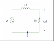
The first order ordinary differential equation that describes a simple series electrical circuit with a resistor, inductor, and sinusoidal voltage source is as follows:
basic methods are distinguished by whether or not they use
L di dt
10 sin(150 t)
iR,
i(t) 0.
(8)
previously computed quantities such as yn-1 , yn-2 , …If they do,
they are called methods with memory and otherwise, one-step![]()
methods.
For this example, the inductance, L is 1 henry and the resis-
tance R is 10 Ω. The voltage source is sinusoidal with a peak
voltage equal to 10 volts and an angular velocity of 150
y(a) A.
(5)
rad/sec. Fig. 1 below gives a pictorial view of the typical cir-![]()
![]()
The computation of yn+1 is often described as taking a step of size hn = tn+1 – tn from tn . For brevity we generally write h = hn in discussing the step from tn. On reaching (tn, yn), the local solution u(t) is defined as the solution of
cuit arrangement in consideration.
u f (t, u)
u(t n )
yn .
(6)
A standard result from the theory of ODEs states that if v(t)
and w(t) are solutions of (3) and if f(t, y) satisfies a Lipschitz![]()
![]()
![]()
![]()
![]()
![]()
condition with constant L, then for α < β we have![]()
v( )
w( )
v( )
w( ) eL( ) .
(7)
In the classical situation that L(b − a) is of modest size, this re-
sult tells us that the IVP (1), (4) is moderately stable. This is
only a sufficient condition. Indeed, stiff problems are (very)
stable, yet L(b − a) >> 1. Without doing some computation, it is
not easy to recognize that a stable IVP is stiff. There are two
essential properties that will help you with this: A stiff prob-
lem is very stable in the sense that some solutions of the ODE
starting near the solution of interest converge to it very rapid-
ly (―very rapidly‖ here means that the solutions converge over
a distance that is small compared to b − a, the length of the interval of integration). This property implies that some solu- tions change very rapidly, but the second property is that the solution of interest is slowly varying.
The basic numerical methods approximate the solution only on a mesh, but in some codes – including all of the MAT- LAB solvers – they are supplemented with (inexpensive) me- thods for approximating the solution between mesh points. The backward differentiation formulas (BDFs) are based on polynomial interpolation and so give rise immediately to a continuous piecewise polynomial function S(t) that approx- imates y(t) everywhere in [a, b]. There is no natural polynomial interpolate for explicit Runge–Kutta methods, which is why such interpolates are a relatively new development. A method that approximates y(t) on each step [tn , tn+1] by a polynomial that interpolates the approximate solution at the end points of the interval is called a continuous extension of the Runge–Kutta formula.
This paper will examine 4 simple applications, one each in electrical, mechanical, chemical and a stiff problem. All solu- tions to the selected problems will require the solution of a differential equation. First, the authors will present a method using the symbolic processing capabilities of MATLAB to
Fig.1 Series RL circuit.
The MATLAB statement written to solve (8) symbolically (i.e., obtaining exact solution) is as follows [2]:
c=dsolve('Dc=-10*c+10*sin(150*t)',' c(0)=0',…
'IgnoreAnalyticConstraints','none')
ezplot(c,[0 0.5])
The dsolve function symbolically solves the ordinary differen-
tial equation specified above. The first argument is the actual
ODE to be solved. D denotes differentiation with respect to the independent variable which in this case is time t. A repeated differentiation process would be required if a digit other than
1 were to follow D. The character following the D (I in this
case, is the circuit current), is the dependent variable. The re- maining terms of the equation are coded as usual. The second
argument is used to specify the initial conditions of the circuit. The initial current in this circuit at t = 0 is 0. The final argu- ment is used to specify the independent variable (missing, MATLAB assumes t by default). Note that all arguments must be contained within single quotation marks as shown. The output from the dsolve function is the symbolic solution to the differential equation.
Next, the differential equation describing the RL electric-
al circuit is modeled using Simulink. Simulink is a block dia-
gram programming language that is packaged with MATLAB.
With Simulink, the differential equation is described using blocks from Simulink library. The blocks include an integra- tor, gain, summer, sine wave source, and scope. The blocks are then ―wired‖ together to generate the differential equation. The complete Simulink model for the electrical circuit is de-
IJSER © 2012
The research paper published by IJSER journal is about Ordinary Differential Equations: MATLAB/Simulink® Solutions 4
ISSN 2229-5518
picted in Fig. 2. Note that a time clock is added to the Simu- limk model to enable the exportation of the simulation time to MATLAB workspace for accesability to plot simulation time against the current.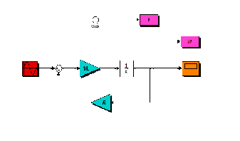
Fig. 2 Simulink model of the RL circuit.
In Simulink, there lies the easy to try different solvers during Simulation. Categorically, a solver in the class of fixed-step solvers and that of the variable step-solvers can be selected. Thus, in this paper, for the Simulink simulation we used the fixed-step solver ode4.
Thus, the graphical result to the RL circuit problem as de-
scribed by (8) is depicted in Fig. 3. It is interesting to note that
ode45 and ode113 (adaptive-step solvers) gave a better approx- imation of the dynamic system compared to ode4 (a fixed-step solver). We decided to capture just one of the points of dispar- ity by zooming the graphical solutions to make our case.
ini_i=0; [t,i]=ode45(@rhs,t,ini_i); plot(t,i,'o'),grid xlabel('t'), ylabel('i')
axis ([0 0.5 -0.1 0.15]) function didt=rhs(t,i) didt=(10*sin(150*t)-i*10)/L; end
end
Given the linear single-input, single-output, mass-spring- damper translational mechanical system, as shown in Fi.g 4. The mathematical model is given as in (9); a second order dif- ferential equation.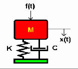
Fig. 4 Mass-spring-damper system.![]()
![]()
![]()
![]()
![]()

For this system, the input is force f(t) and the output is dis- placement y(t), ẏ (t) is the velocity of the system dynamics. Where, c is the damping coefficient and k the spring constant.
my(t)
cy(t)
ky(t)
f (t),
y (t )
0, y(t ) 0.
(9)
Fig. 3 Graphical result of the RL circuit dynamics.
Here, for this example, the m-file option of the model solu- tionhe the following code were used to generate results for the solver ode45:
function RL_ode45_sln t=[0 0.5]
L=1; R=10;
Typically, the suspension mechanisms of automobiles are
modeled as given in (9). For this example the following values were adopted; mas, m=2kg, initial velocity, ẏ =0m/sec, initial displacement, y=0m, damping coefficient, c=2, spring constant, k=4 and f(t)=1.
It is obvious that the dynamic system described by (9) has two states (displacement and velocity), for this research our investigation will focus only on position for obvious reasons. To explore the behavior of the mechanical system, first from the standpoint of the exact solution, the following MATLAB code were used [3]:
y=dsolve('D2y=-(2/3)*Dy –
(4/3)*y + 1/3', 'Dy(0)=0','y(0)=0',...
'IgnoreAnalyticConstraints','none')
pretty(y)
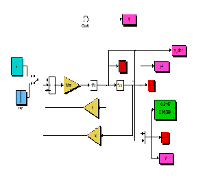
We proceeded to model the system given in (9) in Simulink,
and employed the solvers ode4 and ode45 and ode113 for simu-
lation result. Simulink model of the system is depicted in Fig.
5. Notice also that a both states of the dynamic system are
made available separately in individual scoop blocks and also
in a display block. A third ‗scoop‘ block is also used to display both states in one graph for perusal.A display block shows the numerical values of each state at each time inatant during si- mulation and only the values at the last time of simulation
remains displayed after simulation.
IJSER © 2012
The research paper published by IJSER journal is about Ordinary Differential Equations: MATLAB/Simulink® Solutions 5
ISSN 2229-5518
regime of simulation. Hence, only one of the results is de- picted in Fig. 6.
4.1 Simulation in State-space.
![]()
![]()
![]()
![]()
It is of great importance to also show that the model given in (9) could be formulated in terms of state-space. The model in state-space can be easily mapped in Simulink environment for numerical simulation. This provides the bases for modeling higher order differential equations. For the mass-spring- damper problem, the model for the system is state-space is as given
x Ax
Bu, y
Cx Du.
(10)
Fig. 5 Simulink model of mass-spring-damper system.
To investigate further for comparison, the solver ode45 was employed using the option of MATLAB code to generate the predicted approximate behavior of the system. These codes are:
function spring_mass_damper_ode45 t=[0 6]; % time scale
For the numerical simulation in Simulink, a state-space block
is available in Simulink library. This block allows the direct
input of the A, B, C and D matrixes that are unique to a partic-
ular state-space model. Modern Control Theory has state-
space as its mathematical base [4], hence effective simulation
of state-space models is of paramount importance to the con-
trol and stability engineer, a typical case is dealt with in [5].
4.2 Simulation in Transfer Function.
Also, Simulink gives a flexible platform that allows simulation of dynamic systems in transfer functions. For the mass-spring- damper problem, it can be shown that the equivalent model for (9) in transfer function is as given (11). Simulink has a standard block that allows the direct input of numerator and denominator terms that describe a dynamic system. For clas- sical controller design and analysis [6], this MATLAB capabili-
u=1;![]()
![]()
ty is most adequate.
1 2
![]()
) 1 .
ini_y=0; % initial conditions
x(s) f (s)
(ms
![]()
![]()
cs k
(11)
ini_dydt=0; [t,y]=ode45(@rhs,t,[ini_y; ini_dydt]); plot(t,y(:,1));
function dydt=rhs(t,y)
dydt_1=y(2);
dydt_2=-(2/3)*y(2)-(4/3)*y(1)+ (1/3)*u;
dydt=[dydt_1;dydt_2];
end
end
Note, that either Simulink or MATLAB code could be used to
solve ODEs with any solver of one‘s choice, depending on
which means is more convenient for the user of MATLAB [3].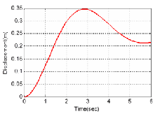
Fig. 6 Mass-springe-damper dynamics solution.
For the ongoing example, ode45, ode113 and ode4 gave a very good approximation of the dynamic system throughout the
The state-space model and transfer function describing the
mass-spring-damper problem modeled in Simulink is shown
in Fig. 7.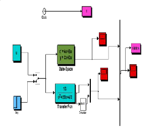
Fig. 7 State-Space and Transfer function Simulink model.
![]()
![]()
![]()
![]()
The following 3 set of ordinary differential equations describes the change in concentration between three species in a tank.
d dt
IJSER © 2012
k1 ,
(0) 5.
The research paper published by IJSER journal is about Ordinary Differential Equations: MATLAB/Simulink® Solutions 6
ISSN 2229-5518
![]()
d dt
![]()
![]()
![]()
k1 k11 ,
![]()
![]()
(0) 0.
(12)
grid
d dt
k11 ,
(0) 0.
function dcdt=rhs(t,c)
The reactions α → β → λ occur within the tank. The constants
k1, and k11 describe the reaction rate for α → β and β → λ re- spectively. Where, k1=1hr-1 and k11 =2hr-1.
For the dynamic system in (12), as earlier done, we seek its
true solution by solving it analytically with the following
MATLAB command.
[a,b,g] = dsolve('Da = -1*a', 'Db = 1*a - 2*b',...
'Dg=2*b','a(0) = 5, b(0) = 0','g(0)=0',
'IgnoreAnalyticConstraints','none')
pretty(a), pretty(b), pretty(g)
ezplot(a) hold on ezplot(b) ezplot(g) Grid on axis([0 5 0 5])
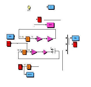
Now we will go ahead to model (12) in Simulink for the sole purpose of obtaining the first numerical solution using the approximation method of ode4 (Runge-Kutta). This was easily modeled as depicted in Fig. 8.
% c(1)=Ca, c(2)=Cb, c(3)=Cg
dcdt_1=-k1*c(1);
dcdt_2=k1*c(1)-k11*c(2);
dcdt_3=k11*c(2);
dcdt=[dcdt_1;dcdt_2;dcdt_3];
end
end
Just like the situation in Fig. 6, no noticeable difference was
observed between the exact result and those of ode45, ode113
and ode4 numerical approximation methods. Hence, a com-
parative plot between them will not reveal anything.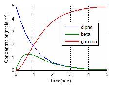
Fig. 9 Concentration of three species dynamics.
![]()
![]()
Stiff ODEs are evil. Most of numerical methods for solving ordinary differential equations will become unbearably slow when the ODEs are stiff. Unfortunately, a large set of ODEs are frequently stiff in practice. It is very important to use an ODE solver that solves stiff equations efficiently. "Stiffness" is associated with equations which have more than one time scale of interest. A stiff ODE is an ordinary differential equa- tion that has a transient region whose behavior is on a differ- ent scale from that outside this transient region. An important characteristic of a stiff system is that the equations are always stable, meaning that they converge to a solution.
y 1000y,
y(0) 1.
(13)
Fig. 8: Simulink model of chemical mixture dynamics.
Finally, for this example we will employ a MATLAB code that will involve the solver ode45 to solve the problem at hand. This was achieved with the following code:
function chem_mixture_ode45 t=[0 5]; % time scale
k1=1;
k11=2;
c0=[5 ;0 ;0]; % initial conditions;
[t,c]=ode45(@rhs,t,c0);
%plot(t,c(:,1),'+',t,c(:,2),'*',t,c(:,3));
plot(t,c(:,1),t,c(:,2),t,c(:,3));
legend('alpha','beta','gamma')
xlabel('Time(seconds)')
ylabel('concentration of each specie(mols/hr)')
Basically, stiff ODE‘s are the motivation for Implicit Methods. Consider a typical example as given in (13). This we will try obtain a solution for it from, first of all the analytical stand- point and the following MATLAB code helped us to do just that.
y=dsolve('Dy=-1000*y', 'y(0)=1',
'IgnoreAnalyticConstraints','none')
The analytical result of (13) is y=e-1000t. The large negative fac-
tor in the exponent is a sign of a stiff ODE. It means this term
will drop to zero and become insignificant very quickly.
For the numerical solution, it is much obvious that ode4, a
fixed-step solver will be a bad choice to approximate a solution
for this model. As a result of the exponent growing, the time-
step must shrink to give acceptable results. In the worst case,
you would have to make your time-step so small that simula-
tions would appear to be stopped. This was a typical expe-
IJSER © 2012
The research paper published by IJSER journal is about Ordinary Differential Equations: MATLAB/Simulink® Solutions 7
ISSN 2229-5518
rience we had when we model (13) in Simulink and tried solve with ode4. As a matter of fact, the simulation went through but no result was displayed graphically (y=1). Interestingly, ode45 gave a very good approximation of the model. The MATLAB code for the ode45 solution is as given below.
function stiff_ode_code
%t=0:0.01:0.4
t=[0 0.006]
ini_y=1;
[t,y]=ode45(@rhs,t,ini_y);
%[t,y2]=ode4(@rhs,t,ini_y);
y_true = exp(-1000*t); % exact soln
%plot(t,y,'o',t,y_true,t,y2,'+'),grid plot(t,y,'o',t,y_true),grid,xlabel('t'), ylabel('y') function dydt=rhs(t,y)
dydt=-1000*y;
end
end
ode45 is based on an explicit Runge-Kutta (4,5) formula, the
Dormand-Prince pair. That means that the numerical solver
ode45 combines a fourth order method and a fifth order me-
thod, both of which are similar to the classical fourth order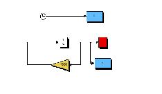
Runge-Kutta method discussed above.
Fig. 10 Simulink model of a typical stiff ODE.
The modified Runge-Kutta varies the step size, choosing the step size at each step in an attempt to achieve the desired ac- curacy. Therefore, the solver ode45 is suitable for a wide varie- ty of initial value problems in practical applications. In gener- al, ode45 is the best function to apply as a ―first try‖ for most problems.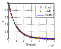
Fig. 11 Stiff ODE solution.
The solver ode45, ode113 and ode15s (stiff solver) gave a good of the model with no obvious disparity. In most cases simulation
of a stiff ode with a non-appropriate solver will be
unnreasnably slow. Fig 11 above gives the simulation results excluding that of ode15s.
In this paper, the authors presented a variety of methods us- ing MATLAB/Simulink to solve Ordinary Differential Equa tions (ODEs). An example problem for each of three engineer- ing disciplines has been provided with that of a typical stiff ODE example. With the RL filter and stiff ODE, we were able to prove the fact no single numerical method of solving a model suffices for all systems. This could be clearly seen in Fig. 3 that the fixed-step solver (ode4) gave a poor approxima- tion of the system at some regimes of simulation. With, the stiff ODE, ode4 failed completely!
The variable step-solvers (ode45 and ode113) gave acceptable results. Thus, identifying the nature of an ODE is the very first step in obtaining its solution. With the mechanical and chemi- cal engineering examples, there was excellent correlation with both fixed-step and variable-step solvers in the results for the three techniques employed, namely: using the MATLAB sym- bolic solver (dsolve) for analytical solutions, using the block diagram programming language-Simulink, and finally using a script file (m-file). With a minimal amount of effort, these techniques allow scientist to solve engineering problems with an excellent ―graphical picture‖ of the result.
The very essence of comparing simulation results with ana- lytical one is to ensure that the numerical approximation gives an acceptable result using the analytical one as a benchmark.
The authors will like to appreciate the Director-General of NASRDA, Dr. S. O Mohammed for making CSTP the bedrock of scientific research in NASRDA. We also thank Dr. Femi A. Agboola, Director, Engineering and Space Systems (ESS) at NASRDA, for his invaluable insight.
[1] L. F. Shampine, I. Gladwell, S. Thompson. Solving ODEs with MATLAB, ISBN 978-0-511-07707-4, USA, 2003.
[2] The MAthWorks, Inc., MathWorks Documentation-MALAB Version
7. Symbolic Math Toolbox,2012.
[3] Delores M. Etter. Engineering Problem Solving with MATLAB‖,
Second Edition Prentice Hall, ISBN-13:978-0133976885, USA,1996.
[4] Robert L. Williams II, Douglas A. Lawrence. ‗Linear State-space Con- trol Systems‘. John Wiley & Sons, Inc. ISBN: 978-0-471-73555-7, New Jersey, USA, 2007.
[5] Aliyu Bhar Kisabo, Femi Agbola, Adetoro Moshood Adesoye Lanre and Ogun Funmilayo Adebimpe. Autopilot Design for A Generic Based Expendable Launch Vehicle, Using Linear Quadratic gaussian (LQG) Control. European Journal of Scientific Research, Vol.50, No.4, (February), pp. 597-611, ISSN 1450-216X,2011.
[6] Aliyu Bhar Kisabo. ―Expendable Launch Vehicle Flight Control; D e- sign & Simulation With Matlab/Simulink‖, ISBN 973-3-8443-2729-8, Germany, 2011.
IJSER © 2012