International Journal of Scientific & Engineering Research, Volume 4, Issue 11, November-2013 359
ISSN 2229-5518
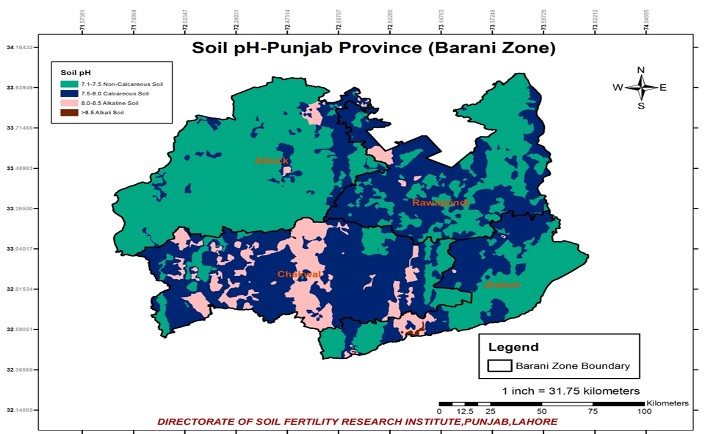
MODELING OF SURFACE SOIL pH USING GEOSTATISTICAL METHODS IN PUNJAB PROVINCE, PAKISTAN
S.M. Mehdi1, S. M. Mian2, S.Ghani1, M. Khalid1, A. A.Sheikh1, S. Rasheed1, M. A. J. Iqbal1
1 Soil Fertility Research Institute, Punjab, Lahore, Pakistan
2 Fatima Fertilizer ( pvt.) Limited
The objective of this study was to evaluate the spatial variability of soil pH by using some interpolation methods such as Kriging, IDW, RBF and splines with the several models and techniques. Soil of the Punjab Province was sampled with respect to the five major crop zones which were Cotton Zone, Rice Zone, Central Zone, Thal Zone and Barani zone. Fom these zones 72,294 soil samples were collected and analyzed. Generating prediction maps of soil pH were conceptualized to correct conventional practices of growing crops .The range of pH in cotton Zone was relatively high as compared with other zones. Muzaffargarh and DG Khan Districts showed high range of pH 4.75 (6.10 to 10.85) and 4.65 (5.65 to 10.30), respectively. The minimum range of pH showed in Attock District which was 1.22 (7.0 to 8.22). The interpolated maps by applying Ordinary Kringing showed the opti- mum variability of soil pH at small scale as compared to other methods and were found that kriging is most suitable method for the estimation of soil pH due to the semi-variogram analysis and it showed highest precision and minimum error. Approximately all districts showed 5% or less CV which showed good method performance.
Keywords: GIS Mapping, Interpolation, Alkaline Soil, Ordinary Kriging, RBF, IDW, Splines, Punjab
Agricultural Land, Semivariogram, Soil pH.
Corresponding Author S. M. Mehdi, Soil Fertility Research Institute, Lahore, Pakistan
E mail: mehdi853@hotmail.com
![]()
Spatial variability of soil pH plays a central role in the devel- opment and management of farming. “Soil pH may vary dra- matically over very small distances (millimeters or smaller), (Brady & Weil, 2010)”. The utility of geostatistics as it relates to farming can be very impressive. “Initially, the main objec- tive of geostatistics in soil science was to enhance the quality of spatial prediction of soil properties” Kuzyakova et al. [6] Variations in soil are recognized for centuries and taken into account of farmer for the maintenance and quality control for getting an optimum yield of suitable crops. In recent times, there is a need to get realize that the variations in soil are sub-
stantial. For better management of land and make optimum use of fertilizers and other agrochemicals, modern techniques and methodologies can be used in order to increase the yields. This realization has lead to better understand the agricultural land precisely and the need to map the soil variations with respect to its different attributes.
As we cannot measure the soil everywhere, there is a need to measure the soil with planned sampling scheme for getting quantitative information from these measurements. Effectively assess the spatial distribution of soil and its variability with respect to parameters, geo-statistic techniques are most com-
IJSER © 2013 http://www.ijser.org
International Journal of Scientific & Engineering Research, Volume 4, Issue 11, November-2013 360
ISSN 2229-5518
monly used in recent years. It provides statistical tools in or- der to find out spatial dissemination of soil and its prediction. Not only the interpolated maps are produced by using these techniques but it also finds error or surfaces which are uncer- tain. This research output would help a lot to bridge over the gap between existing and potential yield level through explo- ration of scope of area-wise crop specialization. Poshtmasari et al. [11] used the geostatistical techniques and methods such as Kriging, Radial basis function, Inverse distance weighted to estimate the soil EC & pH in agricultural land of their study area. It was found that kriging (spherical method) performed well and give optimum results to find out pH because it had lowest error and highest precision. Also RBF was found the most unsuitable method for the estimation of these soil prop- erties. Webster and Oliver [13] discussed the logarithmic transformation techniques to make the respective data normal in behavior. He also described the descriptive statistics and interpolation techniques for the estimation of different proper- ties or parameters. Goovaerts [2] described the recent innova- tion in geostatistics domain and implemented it on the soil scienes. To find out spatial patterns of soil properties, he de- scribed descriptive tools to characterize the semivariogram. Lark [7] described the study of variogram with distinct lag to estimate the soil properties. He also suggested appropriate models that best fitted for the measurements. McDonnell [9] described the phenomena of neighboring measured points that the predicted values get high weights when they are clos- er to its surroundings as compared to the un-sampled values that are far away to its neighborhood. Johnston et al. [3] de- scribed the geostatistical techniques with different methodol- ogies to explore and evaluate the data statistically. They also conclude that soil parameter estimation would be better un- derstood by applying the cross-validation test and RMSE sta- tistics. Robinson and Metternicht (2006) used the different in- terpolation methods like kriging. IDW, RBF to compare the accuracy between them for estimating the soil EC, pH etc. They conclude that many parameters would be better identi- fied from the RMSE statistic obtained from cross-validation after an exhaustive testing. Mohamed and Abdo [10] dis- cussed the soil properties for agriculture with respect to sur- veying, sampling and mapping point of view. Soil surveying includes GIS and sampling methodology with the help of GPS was found to be effective tool. Kastens and Staggenborg [4] discussed interpolation method Kriging with the Semivario- gram studies, prediction accuracy, and generalizing these re- sults with respect to the dataset. For kriging, the choice be- tween a spherical and an exponential variogram probably is inconsequential. Both behave similarly in terms of predictive accuracy. Zandi et al. [14] used different interpolation meth- ods to find out the spatial variability of soil with specific mod- els and techniques. In order to generate prediction maps, these renowned interpolation techniques characterized the spatial variability with respect to soil paprmeters in different con- texts. Bradley and Weil [1] described the soil properties and the principles that can be used to overcome the degradation of soil for getting a better yield or productivity of natural re- sources than the existing phenomena.
The study area based on the land of Punjab Province of Islam- ic state of Pakistan between 69° 15' 0.7158" to 75° 19' 15.0888" in eastern longitude and 27° 41' 42.3636" to 33° 58' 29.0526" in northern latitude. The total study area of research work was about 205,344 km2 (79,284 square miles). It was divided with respect to five major crop zones of Punjab Province; such as Rice zone, Central zone, Cotton zone, Thal zone and Barani zone. These Crop Zones consisted of 34 districts of Punjab Province.
The soil data regarding sample analysis were taken from Di- rectorate of Soil Fertility Research Institute, Agriculture De- partment, Punjab Lahore with 72,294 sample locations during
2010-13.Grid based sampling plan were designed with 3km ×
3km spacing. Soil samples were collected at 6cm depth to
analyze the pH of soil having an accuracy of about ±5m, geo- referenced by using a Global Positioning System (GPS).These analytical results were linked with the geographical location of samples so that an understandable form of maps are devel- oped for a meaningful purpose such as to find out the spatial dissemination of pH in agricultural land of Punjab province, Pakistan.
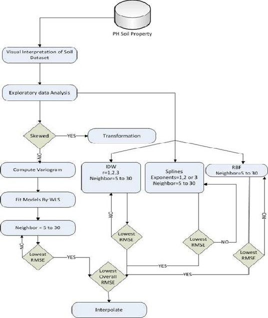
In order to find out the spatial prediction of soil property such as pH on the bases of measured values and for a comparative assessment, methods and techniques were summarized in Figure 2. A manual analysis was conducted to identify outli- ers spatially and incorrect data information by visual interpre- tation and follow ups. Spatial autocorrelation of soil sampled data were also assessed efficiently by this visualization. De- scriptive analysis was also found such as mean, median, min- imum, maximum, standard deviation, skewness, kurtosis and Coefficient of variation in this research. It was also explored with histograms and normal plots. For an efficient assessment of the outlier related values, which were unfavorable for spa- tial forecasting of pH, these tools are useful. In particular, the variogram is very sensitive to detect outliers because it is based on the squared differences among data Lark [7]. If the outlier is closer to the centre of the study area, many times it badly affects the average for each lag.
IJSER © 2013 http://www.ijser.org
International Journal of Scientific & Engineering Research, Volume 4, Issue 11, November-2013 361
ISSN 2229-5518
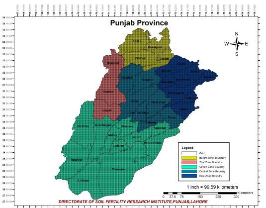
Figure 2.1 Grid Map of Study Area for soil sample location
Apparently, when data tends to behave abnormal, there is a need to transform sampled data to make it normal to some extent. Geostatistical techniques and methods are utilized to get optimum results in this respect.
A logarithmic transformation is considered where the coeffi- cient of skewness is greater than 1 and a square-root
transformation if it is between 0.5 and 1 Webster and Oliver
[13]
Two steps are included in Geostatistical prediction;
1. Identification and modeling of spatial structure
Geostatistical Prediction
2. Variogram is used to study data continuity, its homogene-
ity and the identification of structure spatially.
IJSER © 2013 http://www.ijser.org
International Journal of Scientific & Engineering Research, Volume 4, Issue 11, November-2013 362
ISSN 2229-5518
IJSER © 2013 http://www.ijser.org
International Journal of Scientific & Engineering Research, Volume 4, Issue 11, November-2013 363
ISSN 2229-5518
The presence of a spatial structure where observations close to each other are more alike than those that are far apart (spatial autocorrelation) is a prerequisite to the application of geosta-
average squared difference between the value at z(xi) and the value at z(xi + h) Lark [8];
tistics Goovaerts [2]. The degree of measuring the average dif- ference between the un-measured value and a observed value
γ ( h ) =
N ( h )
[ z ( x ) − z( x
+ h)]2
which is closer or in neighborhood to that un-sampled loca- tion is described by experimental variogram. And thus auto-![]()
2N (h)
∑ i i
i =1
correlation can also be described among sampled data at vari- ous distances. The value of the experimental variogram for a separation distance of h (referred to as the lag) is half of the
where N(h) is the number of data pairs within a given class of
distance and direction. If there exist autocorrelation between
the values at z(xi) and z(xi + h),the results of above equation
will be less with respect to uncorrelated data pair of points.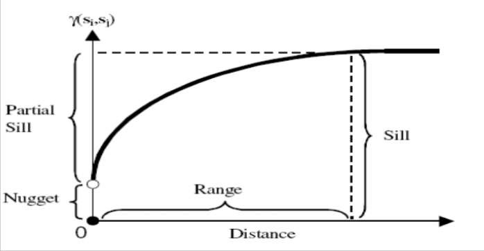
Through the evaluation of experimental variogram, the best fitted model is then chosen such as spherical, exponential etc with respect to weighted least squares and the parameters like sill, range, nugget in this method.
Within a local neighborhood, the average of total weight of measured data points surrounding the un-measured location is actually the value of attribute at that un-sampled location. The equation of this prediction method is given below McDonnell [9];
points within a chosen neighborhood. The weights (r) are re- lated to distance by dij, which is the distance between the pre- dicted point and the measured points. The estimated points that are closer to neighboring measured points get large weights while those has less influence which are far away.
Splines consist of polynomials, which describe pieces of a line
IJSER © 2013 http://www.ijser.org
International Journal of Scientific & Engineering Research, Volume 4, Issue 11, November-2013 364
ISSN 2229-5518
or surface, and they are fitted together so that they join smoothly Webster and Oliver [13]. With the small data varia- tions, the predicted surfaces produce good results but splines are not appropriate for the data that represent high variations within it.
RBF based on the five interpolation techniques which are de- terministic exactly.
1- Thin-plate spline
2- Spline with tention
3- Completely regularized spline
4- Multi quadratic function
5- Inverse multi quadratic function
These interpolators estimate values with respect to measured
values that are identical and surfaces are produced by passing
through each measured point. These predicted values can vary
with respect to the measured values. Total curvature of sur- face is minimized and generation of quite smooth surfaces is based on the predicted values of these methods.
In cross validation mode, mean error and root mean square error is calculated for each model to check the performance of predicted results. Most accurate predictions are shown with the least RMSE.
The Root Mean Square Error was derived according to formula;
[3, 13, 5 and 12]
Cross validation is a technique used to evaluate and validate the developed model of variogram. By removing a subset from the original dataset is required for the prediction or esti- mation of cross validation .This technique is utilized to get the awareness of dataset that which was the best model to be im- plemented in which interpolation method with the appropri- ate neighborhood. These predicted values are compared with measured values to get the least square errors during interpo- lation.
GIS software packages were used to analyze and explore soil sampled data. Maps were developed with ArcMap. Spatial Analyst and Geostatistical Analyst extention are also utilized in this respect. The geostatistical analysis and the statistical approches were carried out using geostatistical extension of ArcMap.
The descriptive statistics of soil pH data such as mean, maxi- mum, minimum, standard deviation, skewness, kurtosis and coefficient of variation is described with respect to the divided zones of Punjab province. Maximum value of soil pH in Rice zone was 10.9 in Hafizabad District.
District | Min | Max | Mean | Median | S.D | C.V | Kurtosis | Skewness |
Lahore | 7 | 10.4 | 8.04 | 8.00 | 0.31 | 3.87 | 6.79 | 1.54 |
Kasur | 7 | 9.9 | 8.07 | 8.10 | 0.27 | 3.29 | 5.00 | 1.13 |
Sheikhupura | 6.2 | 10.3 | 7.96 | 7.90 | 0.34 | 4.33 | 8.53 | 1.58 |
Gujranwala | 6.37 | 10.04 | 7.77 | 7.71 | 0.45 | 5.75 | 3.51 | 1.11 |
Hafizabad | 7 | 10.9 | 8.60 | 8.50 | 0.47 | 5.44 | 2.36 | 0.73 |
Narowal | 6 | 9.65 | 7.69 | 7.77 | 0.53 | 6.91 | 0.62 | -0.38 |
Gujrat | 7.09 | 8.67 | 8.08 | 8.09 | 0.20 | 2.50 | 1.67 | -0.78 |
M.B.Din | 7.02 | 9.1 | 7.85 | 7.90 | 0.28 | 3.59 | 0.10 | -0.02 |
Sialkot | 6.27 | 9.73 | 7.74 | 7.80 | 0.43 | 5.52 | 1.69 | -0.57 |
IJSER © 2013 http://www.ijser.org
International Journal of Scientific & Engineering Research, Volume 4, Issue 11, November-2013 365
ISSN 2229-5518
Approximately mean and median values of soil pH were same in rice Zone of Punjab Province whereas the minimum value
was 6 in Narowal District. Coefficient of variation 5% or less showed good method performance.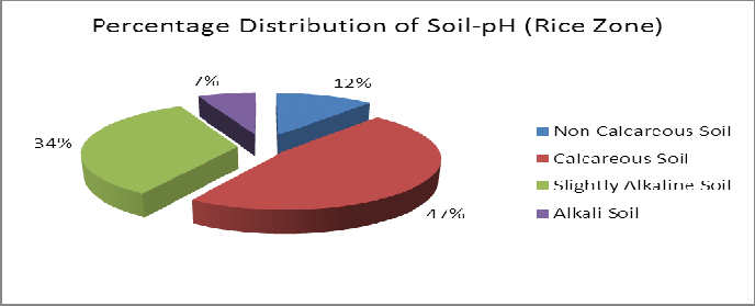
District | Min | Max | Mean | Median | S.D | C.V | Kurtosis | Skewness |
Faisalabad | 7.1 | 10.6 | 7.94 | 7.90 | 0.29 | 3.66 | 14.26 | 2.79 |
Jhang | 7.1 | 10 | 8.03 | 8.00 | 0.37 | 4.56 | 0.62 | 0.57 |
T.T.Singh | 7.2 | 9.7 | 7.88 | 7.90 | 0.23 | 2.97 | 13.46 | 2.19 |
Sahiwal | 7.2 | 9.6 | 8.33 | 8.30 | 0.29 | 3.44 | 1.38 | 0.11 |
Okara | 7 | 10.3 | 8.03 | 8.00 | 0.23 | 2.85 | 11.61 | 1.20 |
Sargodha | 7 | 10.1 | 7.93 | 7.90 | 0.28 | 3.48 | 6.99 | 1.44 |
Khushab | 6.3 | 10.3 | 7.90 | 7.90 | 0.39 | 5.00 | 1.66 | 0.23 |
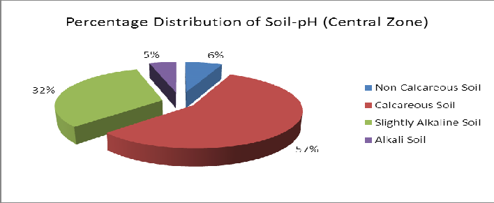
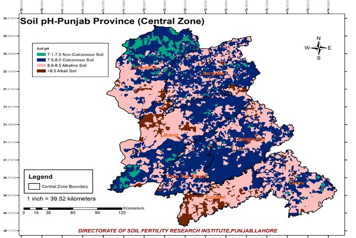
The range of soil pH in central Zone was relatively high in Khushab and Faisalabad Districts that was 4 and 3.5 respec- tively. Maximum value of soil pH in Central zone was 10.6 in
Faisalabad District. Approximately mean and median values of soil pH were same in Central Zone of Punjab Province.
IJSER © 2013 http://www.ijser.org
International Journal of Scientific & Engineering Research, Volume 4, Issue 11, November-2013 366
ISSN 2229-5518
District | Min | Max | Mean | Median | S.D | C.V | Kurtosis | Skewness |
Mianwali | 6.8 | 9.8 | 7.74 | 7.70 | 0.27 | 3.50 | 2.46 | 0.23 |
Bhakkar | 7.09 | 9.5 | 7.76 | 7.70 | 0.19 | 2.48 | 5.46 | 0.93 |
Layyah | 6.29 | 9.46 | 8.14 | 8.16 | 0.27 | 3.30 | 1.32 | -0.53 |
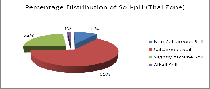
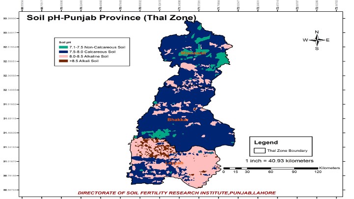
Approximately mean and median values of soil pH were same in Thal Zone of Punjab Province. The range of soil pH in Thal
Zone was relatively high in Layyah District that was 3.17 and the minimum value of soil pH was 6.29.
IJSER © 2013 http://www.ijser.org
International Journal of Scientific & Engineering Research, Volume 4, Issue 11, November-2013 367
ISSN 2229-5518
District | Min | Max | Mean | Median | STD | CV | Kurtosis | Skewness |
Rawalpindi | 6.3 | 8.56 | 7.50 | 7.50 | 0.27 | 3.56 | 2.58 | -0.63 |
Attock | 7 | 8.22 | 7.32 | 7.29 | 0.21 | 2.91 | 1.97 | 1.31 |
Jhelum | 6.1 | 9.2 | 7.46 | 7.40 | 0.32 | 4.26 | 5.61 | 1.46 |
Chakwal | 7.03 | 8.96 | 7.80 | 7.88 | 0.26 | 3.34 | 0.00 | -0.58 |
On the average, the chakwal district had the highest value of soil pH and that was 7.8 and coefficient of variation was 3.34.
The minimum range of pH showed in Attock District which was 1.22 (7.0 to 8.22).
IJSER © 2013 http://www.ijser.org
International Journal of Scientific & Engineering Research, Volume 4, Issue 11, November-2013 368
ISSN 2229-5518
District | Min | Max | Mean | Median | STD | CV | Kurtosis | Skewness |
Multan | 7.8 | 10.7 | 8.62 | 8.60 | 0.33 | 3.81 | 2.02 | 0.36 |
Khanewal | 7.2 | 10.3 | 8.55 | 8.50 | 0.37 | 4.37 | 0.76 | 0.47 |
Vehari | 7 | 10 | 8.31 | 8.30 | 0.33 | 3.94 | 2.93 | 0.94 |
Lodhran | 7.4 | 10 | 8.36 | 8.30 | 0.38 | 4.50 | 1.44 | 0.91 |
Pakpatan | 7 | 8.9 | 8.26 | 8.30 | 0.25 | 2.99 | 0.93 | -0.63 |
D.G. Khan | 5.65 | 10.3 | 7.96 | 7.92 | 0.40 | 5.03 | 5.93 | 1.36 |
Muzaffargarh | 6.1 | 10.85 | 8.28 | 8.20 | 0.47 | 5.69 | 1.51 | 0.82 |
Rajanpur | 6.52 | 8.78 | 7.87 | 7.89 | 0.37 | 4.70 | -0.04 | -0.25 |
Bahawalpur | 7.1 | 9.9 | 8.09 | 8.10 | 0.28 | 3.51 | 1.92 | 0.51 |
Bahawalnagar | 6.1 | 9.8 | 8.06 | 8.00 | 0.27 | 3.31 | 2.68 | 0.46 |
R.Y.Khan | 7 | 10.8 | 8.04 | 8.00 | 0.40 | 4.91 | 9.13 | 2.27 |
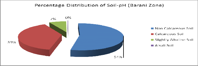
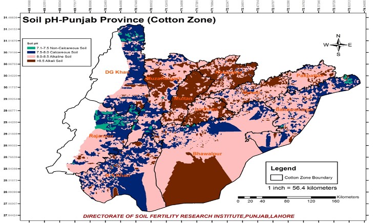
The range of pH in cotton Zone was relatively high as com- pared with other zones. Muzaffargarh and DG Khan Districts
showed high range of pH 4.75 (6.1 to 10.85) and 4.65 (5.65 to
10.30), respectively.
IJSER © 2013 http://www.ijser.org
International Journal of Scientific & Engineering Research, Volume 4, Issue 11, November-2013 369
ISSN 2229-5518
Transformation was done to normalize the values of soil pH of mentioned crop zones of Punjab province. Exploratory Data
Analysis (EDA) of soil pH consisted of statistics and graphical representation of data dissemination. The frequency distribu- tion of soil pH is shown as histogram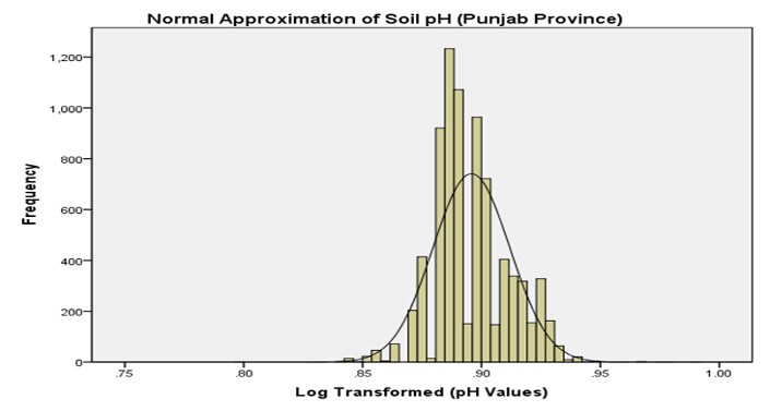
These results indicated that the soil pH data distributed, ap- proximately normal after log transformation. Skewness and
kurtosis results were reduced or controlled with the help of logarithimic transformation.
IJSER © 2013 http://www.ijser.org
International Journal of Scientific & Engineering Research, Volume 4, Issue 11, November-2013 370
ISSN 2229-5518
Method | Model | RMSE |
Ordinary Kriging | Spherical | 0.00217 |
Ordinary Kriging | Exponential | 0.00215 |
Ordinary Kriging | Gaussian | 00.0216 |
Inverse Distance Weighted (IDW) | Multiquardatic | 0.00237 |
Inverse Distance Weighted (IDW) | Inverse Multiquardatic | 0.00214 |
Inverse Distance Weighted (IDW) | Thin Plate Spline | 0,00274 |
Radial Basis Function (RBF) | Power 1 | 0.00297 |
Radial Basis Function (RBF) | Power 2 | 0.00214 |
Radial Basis Function (RBF) | Power 3 | 0,00263 |
Splines | Power 1 | 0.00321 |
Splines | Power 2 | 0.002987 |
Splines | Power 3 | 0.00314 |
It showed that to predict soil pH, Spherical, Gaussian and Ex- ponential models of Kriging (OK) method were chosen for its estimation. And multi-quardatic, inverse multi-quardatic, thin plate spline models of Radial bases function (RBF) were uti- lized. And inverse distance weighted (IDW) method with
suitable first, second and third order polynomial equations were also applied. The highest precision and minimum root mean square error are the basic reason for the prediction of soil pH. These models were analyzed and compared with each other to get the optimum results for best fitted model.
![]()
The study area had different types of soil with respect to pH, which is mainly defined with respect to some ranges as de- scribed below:
Soil Classification of pH | Remarks |
7.5 | Non- Calcareous Soil |
7.5 - 8 | Calcareous Soil |
8 – 8.5 | Alkaline Soil |
≥ 8.5 | Alkali Soil |
IJSER © 2013 http://www.ijser.org
International Journal of Scientific & Engineering Research, Volume 4, Issue 11, November-2013 371
ISSN 2229-5518
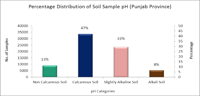
Distribution of soil with respect to pH not only serves as the maintenance and utilization of agricultural land but also provides the quantitative evaluation of soil. Categorically, soil is spatially distributed as shown in table above. Alkaline soil and alkali soil were the major types of soil, which includes
33% and 8% of total surveyed samples, respectively. The soil samples for calcareous soil were relatively higher 47% in Punjab Province than others and non-calcareous were 13% of study area respectively.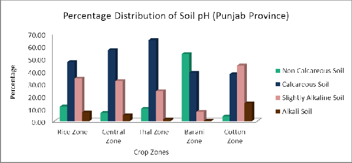
IJSER © 2013 http://www.ijser.org
International Journal of Scientific & Engineering Research, Volume 4, Issue 11, November-2013 372
ISSN 2229-5518
The predicted map of soil pH provides a considerable approach to the agricultural community for the suitable allocation to get a better yield. Because the agricultural land is
degrading due to unawareness of soil and salt concentration problems.
IJSER © 2013 http://www.ijser.org
International Journal of Scientific & Engineering Research, Volume 4, Issue 11, November-2013 373
ISSN 2229-5518

IJSER © 2013 http://www.ijser.org
International Journal of Scientific & Engineering Research, Volume 4, Issue 11, November-2013 374
ISSN 2229-5518
IJSER © 2013 http://www.ijser.org
International Journal of Scientific & Engineering Research, Volume 4, Issue 11, November-2013 375
ISSN 2229-5518
IJSER © 2013 http://www.ijser.org
International Journal of Scientific & Engineering Research, Volume 4, Issue 11, November-2013 376
ISSN 2229-5518

Kriging as a spatial interpolation technique provided the soil structure of pH with unbiased measurements with minimum variance of data. Based on the all zones of pH map,it showed the different concentration of pH. Agricultural land of Punjab province is highly dependent on this soil property. In contrast with other interpolation methods, kriging (Spherical model) provides better estimations approaches for pH soil than the other methods.
Generally kriging is superior with respect to IDW as it gives no assumption about spatial relation and estimated values are incapable of exceeding the value range of sample data. IDW uses a simple algorithm based on distance, but kriging weights come from a semivariogram that was developed by looking at the spatial structure of the data.
It is important to remember that there is no single interpola- tion method that can be applied to all situations. Some are more exact and useful than others but take longer to calculate. They all have advantages and disadvantages. In practice, selection of a particular interpolation method should depend upon the sample data, the type of surfaces to be generated and tolerance of estimation errors. Generally, a three step proce- dure is recommended:
1. Evaluate the sample data to get an idea on how data is distributed in the study area, as this may provide some approach of which interpolation method would be used.
2. Apply an interpolation method which is most suitable in both conditions such as surveyed data and study objec- tives.
3. Comparitive analysis of results would help to find out the best suitable method.
1. Geostatistical analyst provides different interpolation methods with their respective models and techniques for the estimation of soil properties like pH.
2. The predicted measurements using kriging, radial ba- sis function and IDW were compared and evaluate with root mean square error to each other and found that kriging was most suitable for the spatial variabil- ity of soil pH due to the semivariogram analysis.
3. The interpolated maps may help to understand the soil related problem of agricultural land of Punjab provice, Pakistan.
IJSER © 2013 http://www.ijser.org
International Journal of Scientific & Engineering Research, Volume 4, Issue 11, November-2013 377
ISSN 2229-5518
[1] Bradley, N. C. & R. R. Weil. Elements of the nature and properties of soils (3rd Ed.). New Jersey: Prentice Hall, Pub- lishing as Pearson Education, Inc. (2010).
[2] Goovaerts P. Geostatistics in soil science: State-of-the-art and perspectives. Geoderma, 89(1999), 1-45.
[3] Johnston, K.., J.M. Ver Hoef, K. Krivoruchko, and N. Lucas. Using Arc GIS Geostatistical Analyst”, Environmental Systems Research, Redlands, USA. (2001).
[4] Kastens, T. and S. Staggenborg. Spatial Interpolation
Accuracy, Kansas State Precision Ag Conference, January 29-
30, 2002, Great Bend, Kansas.
[5] Krivoruchko, K. and C. A. Gotway. Creating exposure maps using kriging. Public Health GIS News and Information, January Issue. (2004).
[6] Kuzyakova, I. F., V. A Romanenkov, and Ya. V. Kuzyya- kov. Geostatistics in Soil Agrochemical Studies. Eurasian Soil Science, 34(2001), 1011-1017.
[7] Lark, R.M. A comparison of some robust estimators of the variogram for use in soil survey. Eur. J. Soil Sci. 51 (2000a),
137–157.
[8] Lark, R.M. Estimating variograms of soil properties by the
method-of-moments and maximum likelihood. Eur. J. Soil Sci.
51 ( 2000b), 717–728.
[9] McDonnell, R.A and P. A. Burrough. Creating continuous
surfaces from point data. In: Burrough, P.A., Goodchild, M.F., McDonnell, R.A.,Switzer, P., Worboys, M. (Eds.), Principles of Geographic Information Systems. Oxford University Press, Oxford, UK. (1998).
[10] Mohamed, M. and B. Abdo. Spatial variability mapping of some soil properties in El-Multagha agricultural project (Sudan) using geographic information systems (GIS) tech- niques, Ministry of Agriculture and Forestry, Sudan. (2011).
[11] Poshtmasari, H. , Z. Sarvestani, B. Kamkar, S. Shataei, and S. Sadeghi. Comparison of interpolation methods for estimating pH and EC in agricultural fields of Golestan prov- ince (north of Iran). International Journal of Agriculture and Crop Sciences, IJACS 4(2012), 157-167.
[12] Voltz, M. and R. Webster. A comparison of kriging, cubic splines and classification for predicting soil properties from sample information, Journal of Soil Sciences, 41 (1990), 473–
490.
[13] Webster, R. and M. A. Oliver. Geostatistics for Environ- mental Scientists. John Wiley and Sons, Brisbane, Australia.(2001)
[14] Zandi, S., A. Ghobakhlou and P. Sallis. A Comparison of Spatial Interpolation Methods for Mapping Soil pH by Depths, Geo-informatics Research Centre, Auckland University of Technology New Zealand.(2011).
IJSER © 2013 http://www.ijser.org