JEEVAN-KUSHALAIAH METHOD TO FIND THE COEFFICIENTS OF CHARACTERISTIC EQUATION OF A MATRIX AND INTRODUCTION OF SUMMETOR

International Journal of Scientific & Engineering Research, Volume 4, Issue 8, August-2013

ISSN 2229-5518

1553

JEEVAN-KUSHALAIAH METHOD TO FIND THE COEFFICIENTS OF CHARACTERISTIC EQUATION OF A MATRIX AND INTRODUCTION OF SUMMETOR

Neelam Jeevan Kumar [1], Neelam Kushalaiah [2]

[1] Department of Engineering Sciences, Electrical and Electronics Engineering, Jawaharlal Technological

University, Hyderabad, 19-6-194, Rangashaipet, Warangal, Andhra Pradesh, India - 506005. Contact No: +919492907696, Email Id: neelamkushalaiah@gmail.com

[2] Telecom Communications, BSNL, India, 19-6-194, Rangashaipet, Warangal, Andhra Pradesh, India -

506005. Contact no: +918985230271, Email Id: neelamkushalaiah@hotmail.com

Abstract: The method is based on one of the arts of ancient tradition is Basket Weaving registered resolution number: 12011/68/93-BCC( C ) and date 10/09/1993 Andhra Pradesh, India. The method gives maximum number of possible square sub matrices of a square matrix starting from minimum order to maximum order. By this method, coefficients of characteristic equation of a square matrix are calculated. The Summetor symbol is newly introduced. The function of Summetor is same as Factorial instead of multiplication, addition is performed. The method name is named on the authors

Jeevan and Kushalaiah of the article or manuscript.

Keywords: [1] Basket Making, [2] Summetor, [3] J-K chart, [4] Formula of Coefficients

I. Introduction

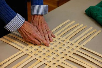
Basket Weaving or Basketry or Basket Making[1] is an art of making thin strips of cane in to a basket or other similar form. Horizontal and Vertical strips are like rows and Columns of a matrix and coordinated position of row strips and column strips gives element position of the matrix.

1 2 3 4 5

Fig.1 Basket maker making a Basket with strips of Cane, 5x5 matrix with 5 Horizontal strips and 5 vertical strips . The dots are the elements which are formed by Coordinates of horizontal and vertical
strips

International Journal of Scientific & Engineering Research, Volume 4, Issue 8, August-2013

ISSN 2229-5518

1554

We know that

|AI − A| = 0 ……………. (i)

The polynomial equation

C0λ n +C1 λ n-1+C2 λn-2+……Cn-1 λ+ Cn = 0 …………………. (ii) SUMMETOR[2]: sum of variable element starting from minimum limit to maximum limit n-times

. n no.of continition summations

P=l

P = P!
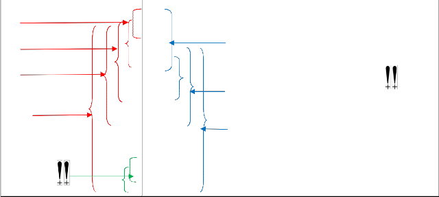
Summetor Symbol

Indicates summation between two integers
Fig 2. Summetor symbol

II. Calculation of Coefficients

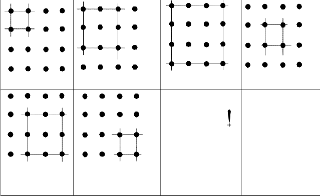
Let us assume that a square matrix-A has n-rows and n- columns. The order of sub matrices is increases from [1x1] to [n-1 x n-1]. Every Coefficient is sum of determinant sub matrices to the order respectively.
Each determinant of sub matrix is denoted by Φj,k
Where j - the order of the sub matrix k - Sub matrix no.

a11 a12

3 a21 a22

a13 … … a1n
a23 … … a2n⎥
= ⎢a31
a32
a33 … … a3n
⎣a : 1 a : 2 : :

1 2 3 ………. n

n n an3 … … ann⎦
Fig.3 Formation of nxn Matrix with n horizontal and vertical strips of cane.

International Journal of Scientific & Engineering Research, Volume 4, Issue 8, August-2013

ISSN 2229-5518

1555

The Important notes of Jeevan – Kushalaiah Method are given below
Notes .1: C0 = 1 …. ( ii.a )
Notes .2: C1 = Trace (A) = sum of diagonal elements = ∑n
aii
…. ( ii.b )
Notes .3: Cn = Determinant of Matrix-A = |A| …. ( ii.c )

Calculation of co-factor C1

Put one horizontal and vertical strip on each diagonal element. Sum the all the determinants of coordinates of vertical and horizontal elements.

No. of coordinative Determinants = n (n – order of the matrix or Trace(A) )

C1 = Trace (A) = ∑n

aii

……… (iii)

1 2 … n

Calculation of co-factor c2

Φ2,2 = a11 a13

a22 a23

Φ 2,1 = a11 a12

a31 a33

Φ2,3 = a11 a1n Φ2,4 =

a21 a22

an1 ann

Where 2K

2,K = (n - 1)

a32 a33

Φ2,5 = a22 a2n Φ2,K =

an2 ann

a n − 1, n − 1 a n − 1, n

a n − 1, n ann

International Journal of Scientific & Engineering Research, Volume 4, Issue 8, August-2013

ISSN 2229-5518

1556

Calculation of co-factor C3

a11

Φ3,1 = a21

a12

a22

a31

a32

Φ3,2

a11

a12

a1n

Φ3,3

a11

a1, n − 1

a1n

a13

a23

a33

= a21

an1

a22

an2

a2n

ann

= an − 1, n an1

an − 1, n − 1

an, n − 1

an − 1, n

ann

Where 3,K

3,K = (n - 2)

Φ3,K

an − 2, n − 2

= an − 1, n − 2

an, n − 2

an − 2, n − 1 an − 1, n − 1 an, n − 1

an − 2, n

an − 1, n

ann

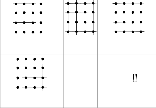
Fig.4 Formation sub matrices with diagonal elements and determinants. J-K sub matrix Equation

ΦS,K = (n - (S-1)) S-1 ……………. ( iv )

The limits of S, 2≤ S ≤ n

Total no. of sub matrices

<IS,K

s=2

(n − (S − 1)) S − l

. …………… ( v )

Every sub matrix should be formed with diagonal elements and respective horizontal and vertical

coordinate elements only.

International Journal of Scientific & Engineering Research, Volume 4, Issue 8, August-2013

ISSN 2229-5518

1557

No. of diagonal elements of a sub matrix is equal to the order of the sub matrix

III. J-K chart[3] with diagonal elements for Sub matrices

Matrix – A has order of nxn i.e., n diagonal elements. From note 2: We know that C1 is Trace(A), ( ii.b )

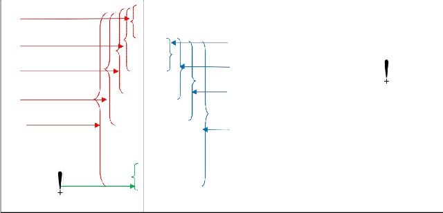
For C2 : Chart of 2x2 Determinant sub matrices

a11

Φ2,1

No . of 2x2 sub matrices

Φ2,2

Φ2,3

Φ2,4

Φ2,n-1

Φ2, n - 1

a22 a33 a44 a55

:

ann

Φ2,n

Φ2,n+1

Φ2,n+2

2,(n - 1)

For C3: Chart of 3x3 Determinant sub matrices

a11

Φ3,1

a22

Φ3,2

a33

3,3

a44

Φ3,n-1

No . of 3x3 sub matrices

3,(n - 2)

Φ3,n-2

Φ3, n - 2

a55

:

a

Φ2,n

Fig .4: Formation of Determinant sub matrices of Cn

International Journal of Scientific & Engineering Research, Volume 4, Issue 8, August-2013

ISSN 2229-5518

1558

The sign of coefficients

Notes .4: If C0 is positive, then Cn = (-1)S …. (vi.a) Notes .5: If C0 is negative, then Cn = (-1)S+1 …. (vi.b) Limits of n, 0 ≤ n ≤ maximum order.

IV. Problem with Explanation

Let a matrix – A order 5x5.

⎤

The characteristic Polynomial equation of the Matrix – A is

|A − AI| = 0

Where I is 5x5 Identity matrix

5 − A 2 2 l 7

9 5 − A 9 8 3

9 9 8 − A

6 5 6

3 6 7

3 − A

2 − A

= 0

The polynomial is, -λ5 + 23λ4 + 98λ3 + 196λ2 + 1099λ + 3017 = 0 …… ( a )

a) Calculation of Characteristic Equation by using Jeevan – Kushalaiah Method

⎤

Given Matrix, A =

Step 1: from equations (ii.a), (ii.b) and (ii.c)

Notes .1: C0 = 1
Notes .2: C1 = Trace (A) = sum of diagonal elements = ∑n
aii
Notes .3: Cn = Determinant of Matrix-A = |A|

International Journal of Scientific & Engineering Research, Volume 4, Issue 8, August-2013

ISSN 2229-5518

1559

C0 = 1,
C1 = Trace(A) = 5 + 5 + 8+ 3 + 2 = 23
Cn = det (A) = |A| = 3017

Step .2: calculate coefficients C2 to Cn-1

Calculation of C2 sub matrices determinants

The maximum no. of 2X2 sub matrices are, i.e., from equation ( iv )

ΦS,K = (n - (S-1)) S-1

Here S = 2

2,K = (n - 1) =

Calculation of C3 sub matrices determinants

The maximum no. of 2X2 sub matrices are

Here S = 3, substituting in equation ( iv )

3,K = (n - 2) = ( 5 - 2) = 3 = 3 +2 +1 =

3+2+1+2+1+1 =10

5 2 2

Φ 2,1 = a11 a12

a21 a22

Φ 2,2 = a11 a13

a31 a33

Φ 2,3 = a11 a14

a41 a44

Φ 2,4 = a11 a15

a51 a55

Φ 2,6 = a22 a24

a42 a44

Φ 2,7 = a22 a25

a52 a55

Φ 2,8 = a33 a34

a43 a44

Φ 2,9 = a33 a35

a53 a55

Φ 2,10 = a44 a45

a54 a55

= 5 7

= 5 8

5 3

= 5 3

6 2

= 8 1

6 3

= 8 5

7 2

= 3 7

8 2

= 10 – 21 = -11

= 15 – 40 = - 25

= 10 – 18 = -8

= 24 – 6 = 18

= 16 – 35 = -19

= 6 – 56 = - 50

Φ3,6 =

3,9

5 2 7

3 7 2

5 1 7

6 3 7

= 32

= 58

International Journal of Scientific & Engineering Research, Volume 4, Issue 8, August-2013

ISSN 2229-5518

1560

Calculation of C4 sub matrices determinants

The maximum no. of 2X2 sub matrices are

C2 = ∑(n − 1)

Φ 2, i = Φ

2,1

+ Φ 2,2 + Φ

2,3 + Φ

2,4+

Here S = 4, substituting in equation ( iv )

4,K = (n - 3) = ( 5 - 3) = 2 = 2 +1 =

Φ 2,5 + Φ 2,6 + Φ 2,7 + Φ 2,8 + Φ 2,9 + Φ 2,10 = 7 + 22 + 9 -

11 -41 -25 -8 + 18 -19 -50 = -98

C3 =∑(n − 2)

Φ 3, i = Φ

3,1 + Φ

3,2 + Φ

3,3 + Φ

2 + 1 +1 = 2 + 1 + 1 + 1 = 5

3,4+ Φ 3,5 + Φ 3,6 + Φ3,7 + Φ 3,8 + Φ 3,9 + Φ 3,10 = -115 -

68 + 215 + 54 +172 + 32 + 4 + 58 + 72 -228 = 196

5 2

Φ4,1 = 9 5

9 9

2 1

9 8 = 5

8 1

C4 =∑(n − 3)

Φ 4, i = Φ

4,1 + Φ

4,2 + Φ

4,3 + Φ

Φ4,2 =

= - 913

4,4+ Φ 4,5 =5 -913 -474 -495 + 778 = -1099

Coefficients with signs:

From note 1, 2, 3 and 5

C0 is negative = (-1)S+1 = -1

5 2 1 7

C1 = (-1)

1+1

3+1

* 23 = 23, C2 = (-1)

2+1

* -98 = 98,

4+1

Φ4,3 = 9 8

1 5 = - 474

C3 = (-1)

* 196 = 196, C4 = (-1)

* 1099 =

6 6

3 7

5 2

Φ4,4 = 9 5

6 5

3 6

5 9

Φ4,5 = 9 8

5 6

6 7

3 7

8 2

1 7

8 3 = - 495

3 7

8 2

8 3

1 5 = 778

3 7

8 2

1099, C5 = (-1)5+1 * 3017 = 3017

Substituting C0,C1, C2, C3 C4 and C5 in equation (ii) We get

-λ5 + 23λ4 + 98λ3 + 196λ2 + 1099λ + 3017 = 0

….. (b)

i.e., (a) = (b)

Hence the method id verified successfully.

The general Formula of Coefficients[4]

Cs =(-1)S ∑

k= n – (S-l) S-l s=n

s=0

k= l

<Is, k

…………… ( vii )

International Journal of Scientific & Engineering Research, Volume 4, Issue 8, August-2013

ISSN 2229-5518

1561

V. Result

Result!

Plots:

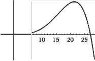
1 X 106

500000

-500000

-1 X 106

(.:\ from -5 to 25)

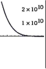
-100 -50 50

-1x1o10

-2 X 1010

p. from -100 to 100)

Alternate forms:

.:\ (.:\ (.:\ (98 -(.:\ -23) .:\) + 196) + 1099) + 3017

.:\ (.:\ (.:\ ((23- .:\) .:\ + 98) + 196) + 1099) + 3017

Fig .5: Result calculated by Wolfram alpha (Oxford) Direct Link of the problem with wolfram alpha: http://www.wolframalpha.com/input/?i=characteristic+polynomiai+%7B%7BS%2C2%2C2%2Cl%2C7%7

0%2C%7B9%2CS%2C9%2C8%2C3%70%2C%7B9%2C9%2C8%2C%l 2CS%70%2C%7B6%2CS%2C6%2C3%2

C7%70%2C%7B3%2C6%2C7%2C8%2C2%70%70

International Journal of Scientific & Engineering Research, Volume 4, Issue 8, August-2013

ISSN 2229-5518

1562

VI. Conclusion

The Jeevan – Kushalaiah Method is used for calculating cofactors of any order square matrix characteristic polynomial equation to find the Eigen values and Eigen vector without using equation no. 1. This is a method based on determinants only. This method is not applied for non square matrices. The calculation and computational time very small for lower order square matrices and as the order of the square matrix increases the computational time increases. It 100 percent applicable method in real world based computational time.

VII. References

[1] Blanchard, M. M. (1928) The Basketry Book. New York: Charles Scribner's Sons

[2] Bobart, H. H. (1936) Basket work Through the Ages. London: Oxford University Press

[3] W.B Jurkat and H.G Ryser, “Matrix factorizasation and Determinants of permanents”, J algebra 3,1966,1-27

Math. 1356, Springer - Verlag, 1988

[4] H. Volkmer, Multiparameter eigenvalue problems and expansion theorems. Lect. Notes.

[5] J. W. Demmel, Applied Numerical Linear Algebra, SIAM, Philadelphia, 1997

[6] L. N. Trefethen and D. Bau, III, Numerical Linear Algebra, SIAM, Philadelphia, 1997 [7] Wikipedia link: http://en.wikipedia.org/wiki/Basket_weaving

[8] Wikipedia link: https://en.wikipedia.org/wiki/Summation

[9] Wikipedia link http://en.wikipedia.org/wiki/Characteristic_polynomial

[10] T.S. Blyth & E.F. Robertson (1998) Basic Linear Algebra, p 149, Springer ISBN 3-540-76122-5 . [11] John B. Fraleigh & Raymond A. Beauregard (1990) Linear Algebra 2nd edition, p 246, Addison- Wesley ISBN 0-201-11949-8

[12] Werner Greub (1974) Linear Algebra 4th edition, pp 120–5, Springer, ISBN 0-387-90110-8