International Journal of Scientific & Engineering Research, Volume 6, Issue 1, January-2015

ISSN 2229-5518

59

Experimental and CFD of Designed Small Wind

Turbine

Tarek A. Mekhail, W. Abdel Fadeel, Walid M. A. Elmagid

Abstract— many researches have concentrated on improving the aerodynamic performance of wind turbine blade through testing and theoretical studies. A small wind turbine blade is designed, fabricated and tested. The power performance of small horizontal axis wind turbines is simulated in details using Computational Fluid Dynamic (CFD). The three-dimensional CFD models are presented using ANSYS-CFX v13 software for predicting the performance of a small horizontal axis wind turbine. The simulation results are compared with the experimental data measured from a small wind turbine model, which designed according to a vehicle-based test system. The analysis of wake effect and aerodynamic of the blade can be carried out when the rotational effect was simulated. Finally, comparis on between experimental, numerical and analytical performance has been done. The comparison is fairly good.

Index Terms— small wind turbine , CFD of wind turbine, CFD, performance of wind turbine, test of small wind turbine, wind turbine aerodynamic, 3D model.

1 INTRODUCTION

——————————  ——————————
lobal warming are the most important problems in today’s world. Fossil fuel prices are increasing very sharply because of limited sources. Natural balance of
earth is changing be-cause of global warming. One of the main reasons of this change is burning too much fossil fuel. There- fore, alternative energy sources are needed Wind is such a resource available that it just blows everywhere, from large areas to local winds it just blows.
Small wind turbines were adapted to be operated in Ken- yan wind climates by Berges [1].An example, well-designed
300W wind turbine can already provide 60% of basic rural Kenyan school electricity needs (2kWh/day) in low wind cli- mate, and up to 90% if the rotor is oversized for the given gen- erator. In high wind climate, the wind turbine would produce much more than the basic needs.
Turbine blades were optimized for the maximum power production for a given wind speed, a rotational speed, a num- ber of blades and a blade radius. Aerodynamic design and op- timization tool for wind turbines is developed by using both Blade Element Momentum (BEM) Theory and Genetic Algo- rithm. The airfoil profiles and their aerodynamic data are taken from an airfoil database for which experimental lift and drag coefficient data are available using in the BEM theory to opti- mized the blade shape configuration .The optimization meth- odology is employed to design a 1MW wind turbine with a 25m radius by Ceyhan [2].
The problem of poor performance of small wind turbine oc- curs as a result of laminar separation and laminar separation bubbles on the blades, caused by the low Reynolds number (Re) resulting from low wind speeds and small rotor size [3]. The use of specially designed low Re airfoils permits start up at lower wind speeds, increasing the startup torque and thus improving the overall performance of the turbine.
Song [4] designed a small wind turbine blade, fabricated and tested in his study. The power performance of small hori- zontal axis wind turbines was simulated in detail using modi- fied blade element momentum methods (BEM). Various fac-
tors such as tip loss, drag coefficient, and wake were consid- ered. The simulation was validated by experimental data col- lected from a small wind turbine having commercial name (Bergey XL 1.0).
Wind turbine simulation through Computational Fluid Dy- namics (CFD) software offers inexpensive solutions to aerody- namic blade analysis problem. Two-dimensional airfoil (i.e. DU-93 and NREL-S809) CFD models were presented using ANSYS-FLUENT software. Using the Spalart-Allmaras turbu- lent viscosity, the dimensionless lift, drag and pitching mo- ment coefficients were calculated for wind-turbine blade at different angles of attack. Optimum values of these coeffi- cients as well as a critical angle were found from polar curves of lift, drag and moment modeling data. These data were ex- ploited in order to select the airfoil with best aerodynamic performance for basis of a three-decisional model analogue [5].
Chick et al [6] developed various models to estimate the wake effect and optimize the sitting of a wind farm. Computa- tional Fluid Dynamics (CFD) has been a useful tool towards the understanding of wake behavior on different terrains such as wind turbine mounted on plains and hills. By using CFD code to study the wake interaction, the optimum distance be- tween adjacent wind turbines can be predicted in different terrains.
3D CFD rotor computations of a Siemens SWT-2.3-93 varia- ble speed wind turbine with 45m blades is carried out by Laursen et al [7].The complex flow associated with the roll up o f tip vortexes and 3D flow at the root sections can be effec- tively visualized with the application of CFD. The results of the two different CFD codes, ANSYS-CFX and Ellipsys were compared with both an in-house BEM code and CFD compu- tations performed by a third party.
In the present study, the 3D model is used to investigate and analyze the flow in the turbine, using ANSYS CFX v13. In other hand, the different program using to carry out wind tur-

IJSER © 2015 http://www.ijser.org

International Journal of Scientific & Engineering Research, Volume 6, Issue 1, January-2015

ISSN 2229-5518

60

bine model by Cao [5], and Laursen et al [7]. The model is car- ried out using personal computer with 5i Core processor. The result compared with data out from experimantal work to
Usually, A2 is replaced with A, U1 is replaced with U, and the performance of a wind turbine is represented by the power coefficient Cp
make model validation.

2 AERODYNAMICS OF HORIZONTAL AXIS SMALL WIND

P

C = 1
2 ρAU
= 4a(1 − a) (4)

TURBINES, DESIGN AND FABRICATION

A wind turbine blade is designed by using Matlab code to solve Blade Element Theory (BET) equations. Blade aerody- namic parameters determination is optimized to close maxi- mum available performance. After the design is completed, The fiberglass used to manufacture the three blades. Finally, the other parts of wind turbine are fabricated and complete wind turbine ready to be tested.

2.1 Small Wind Turbine Aerodynamic

The Blade Element Theory is the most important aerody- namic analysis used to design the wind turbine. The momen- tum theory is roll to the BET. Betz developed a simple model to predict the performance of ship propellers and this model is widely used to demonstrate the principle of wind turbines, which called Actuator Disk theory. He assumed the air was one dimensional, incompressible, and time-invariant, and then
After calculating the derivative of CP to find maxi- mum CP,Max , one could get CP,Max = 0.5926, where a =1/3. This is the Betz limit. No practical wind turbine reaches this limit for it is the theoretically maximum power coefficient.
In Betz analysis, the wake rotation is not considered to influence the airflow. Actually, wake rotation analysis is another method to calculate wind turbine power, and was developed initially by Glauert in 1935. When an annular stream tube at the rotor plane (section 2 and 3 in Fig.1) is tak- en out the thrust on an annular element is dT.
1

dT = (p − p )dA = ρ (Ω + ω) ωr ∙ 2πrdr (5)
2
Where r is the radius of the blade, dr is the thickness; Ω is
angular velocity of the wind turbine rotor, and ω is the angu-
lar velocity of the wind. Similarly, a’ is defined as angular (or
tangential) induction factor, defined as:
with the principle of conversation of momentum in Fig. 1, [4]. In addition, Bernoulli function was applied for sections 1 and
2, 3 and 4 respectively with the assumption that p1= p4 and U2
= U3, thrust on the disk also could be deduced.

ω
a =
2Ω
Substituting Eqn. 5 into Eqn. 6:
(6)
1

� = 𝐴 (𝑝 − 𝑝 ) =
2
�𝐴 (� − � ) (1)
𝑑� = 4�𝑎 (1 + 𝑎 )�𝛺 𝑟 𝑑𝑟 (7)
With the Betz analysis axial momentum also could be de-
fined as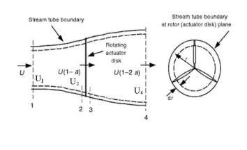

dT = 4 ρU a(1 − a)πrdr (8)
With Eqns. 7 and 8, local speed ratio λr is defined as:
𝜆 =

𝛺𝑟
�

𝑎(1 − 𝑎)
= [
𝑎′(1 − 𝑎 )

] (9)
Fig. 1. Actuator disk model for rotor analysis.
Thus, the axial induction factor, a, is defined as the velocity decrease from section 1 to section 2
U − U
From the conversation of angular momentum, the torque on the annular element is dQ, When Eqns. 2 and 6 are substitut- ed in Eqn. 9,
dQ = dṁ(ωr)dr = 4a (1 − a)ρUπr Ωdr (10)
The forces on the blades of a wind turbine can also be ex-
pressed as a function of lift and drag coefficients and the angle of
attack. The blade is assumed to be divided into N sections, which

a =
U
Then the power P,
1
(2)
are called as blade elements, shown in Fig. 2. To explain Blade El- ement Theory, some assumptions are made. There is no aerody- namic interaction between blade elements. Span wise velocity components on the blade are ignored. The forces on blade element

� = � ∙ � =
2
�𝐴 � ∙ 4𝑎(1 − 𝑎) (3)
are determined solely by the lift and drag characteristics of 2D air- foils of blades.

IJSER © 2015 http://www.ijser.org

International Journal of Scientific & Engineering Research, Volume 6, Issue 1, January-2015

ISSN 2229-5518

61

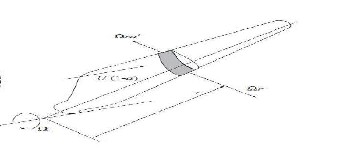
Fig . 2. Definition of blade element used in the theory.

In the blade element analysis, lift and drag compo- nents are perpendicular and parallel to the relative wind speed direction. Consider a turbine with N blades of tip radius R, each with chord length c and set ϕ pitch angle measured between the airfoil zero lift line and the plane of the disc. Chord length and pitch angle may vary along the blade span. As shown in Fig. 3, the following relationships among the pa- rameters can be determined as below.
In Figure 3, θp is section pitch angle, θp,0 is blade pitch angle at the tip, θT is section twist angle which is defined relative to the tip, α is the angle of attack and ϕ is the angle of relative wind. dFL is the incremental lift force, dFD is the incremental drag force, dFN is the incremental force normal to the plane of rotation (related to thrust), and dFT is the incremental force tangential to the circle swept by the rotor, which contributes to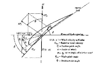


Fig . 3. Blade geometry for analysis of wind turbine [4], study from Wind Atlas for Egypt [8]) and then the geometry
of the blade. Defining the operating conditions at which the
blade is designed is a key first step. Indeed CL (α, Re) and CD
(α, Re) are function of α, Re function, themselves function of respectively Uin , Ω and the twist angle θ for the former and
Urel and the chord length c for the later.
Once those design parameters have been determined,
the procedure consists in maximizing the expression:
f(a, a ) = a (1 − a) (15)
From Eqn. 9 a’ is a function of a, thus for a given r the problem
reduces to seeking the (a, a’) combination yielding df/da = 0.
the useful torque, Urel is the relative wind velocity, U(1-a) is wind velocity at blades
df da


= (1 − a) − a ⇔
da da


da a
= (16)
da 1 − a
∅ = tan [

1 − a
(1 + a )λ_r
] (11)
Another expression for da’/da is provided by differentiating
Eqn. 9 with respect to which yields:

U(1 − a)
U =
sin ∅
(12)

da′
=
da

1 − 2a
(1 + 2a )λ
(17)
If the rotor has B blades, the total normal force on the local
radius r is,

U (1 − a)
And replacing λ2 in Eqn. 17 to Eqn.9 yields to the final relation- ship between a and a’:
dF = σπρ
sin θ
(C cos ∅ + C sin ∅)rdr (13)

1 − 3a
a =
(18)
The differential torque from the tangential force at local radius
r, is,
4a − 1
𝑑� = 𝜎��

� (1 − 𝑎)
sin 𝜃
(𝐶 sin ∅ − 𝐶 cos ∅)𝑟 𝑑𝑟 (14)
Combining Eqn. 18 and Eqn.9 yields the optimum relationship between a and λ:

2.2 Blade Design for Maximum Power Production

Performance

The methodology of designing a blade for maximum power performance consists first in determining the design operating conditions (defined with Uin and Ω) which depend- ed on weather of operation area (Taken Aswan weather in this
16a − 24a + a(9 − 3λ ) − 1 + λ = 0 (19)
Once this relationship is satisfied, the flow angle can be de-
rived as:

1 − a
tan ∅ = (1 + a )λ (20)

IJSER © 2015 http://www.ijser.org

International Journal of Scientific & Engineering Research, Volume 6, Issue 1, January-2015

ISSN 2229-5518

62

Prior to compute the optimum local twist angle θopt, the airfoil must be selected and the optimum value for the local angle of attack αopt must be determined. The goal is to maxim- ize the tangential force, or its dimension-less value (Ct). Due to the Reynolds dependency for CL and CD, Uin and Ω are not enough to calculate Re but the chord length copt is also needed. Therefore, computing αopt and copt are within this methodolo- gy interconnected. It means that a first value for αopt is derived based on Re guess. Then this first value for αopt will be in- putted to compute copt, and back this copt value will be used to recalculate Re, and so on until all values converge. On a loop process, both αopt and copt are derived

2.3 The Small Wind Turbine Blade Design Result

The small wind turbine is developed to match the local weather conditions (Aswan city), by using The Blade Element Theory (BET). The blade design is the most important and the key of capture wind power. The following main deign param- eters are entered to BET code implemented by using Matlab.

 Wind speed is 3 m/s taken from wind atlas [8], (Uin = 3m/s).

 Wind turbine shaft speed is 150 rpm (Ω=150 rpm).

 The blade radius is 1.1m limited by manufacturing

consideration(R=1.1 m).
From these parameters , the tip speed ratio (λ) is calculated
and have value λ = 5.7596, which in range of optimum value
found in many researches, Vitalea and Rossib [9] ,Singh et al
[3] and song [4] . The value of desgined λ limits rotation shaft speed. Because of high shaft speed need more specific manu-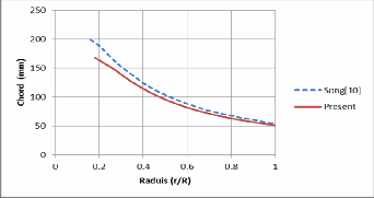

facture consideration, which hard to do it.The air physical pa- rameter also was needed, that was taken constant in the pre- sent work. The airfoil is selected to be easy to manufacture, so NACA 4412 is used. The resultant of chord distribution and twist angle are shown in Fig. 4 and Fig. 5, respectively. Song [4] develops his small wind turbine at close dimension range, so comparison between the chord distribution and twist angle resulted with song’s result is done. The Fig. 4 and Fig. 5 are illustrated similar trend. However, the deviation in twist angle and chord distribution found due to different operating condi- tion.

Fig. 5. Small wind turbine blade twist angle.

2.4 Wind Turbine Fabrication and Test

The dimensions of the blades are calculated by using Matlab code to solve the Blade Element Theory equation. The chord distribution and twist angles at different radii are shown in Fig.4 and Fig. 5. These dimensions are used to fabri- cate the blades. The wind blade turbine is most important and expensive part in wind turbine, due to complicated shape.
The following procedures are done to make blade mold which using for molding three blades, to ensure that three blade are identical.

 Cutting the airfoil in different section with suitable cord in tough material

 Adjust the dimension of space and height from ref- erence surface to match Blade Element Theory da- ta.

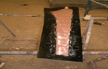
 Fill the space by paint paste that make blade die. It guides to mold, as shown in Fig. 6.

 Make the wind blade mold from the rubber and

just clearance to match airfoil shape.



Fig. 6. The guide of the blade dies
Fig . 4. Chord distribution of small wind turbine.
The blade mold is ready to make fiberglass wind turbine. It has full blade dimension, obtained from Matlab code. The oth- er common step to fabricate the wind turbine blade is done to produce the blade from raw material. The fiberglass blade manufacturing procedure carries under supervisor of produc-

IJSER © 2015 http://www.ijser.org

International Journal of Scientific & Engineering Research, Volume 6, Issue 1, January-2015

ISSN 2229-5518

63

tion engineer specified in fiberglass production in specialist factory using the mold. Fig. 7 shows the final mold and wind turbine blade.


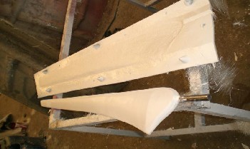
Fig. 7. Final shape of the mold and wind turbine blade

After that, the three blades, hub, generator and tower are assembled. Final wind turbine model is shown in Fig. 8.
The wind turbine is installed on a tower that is fixed to a truck or trailer. The performance of the turbine can be meas- ured across a full range of wind speeds by driving the vehicle at different speeds on a controlled course. This method is a rapid testing approach that can be used to rapidly evaluate performance with relatively low costs. Vehicle based testing was chosen to validate the present turbine to get its perfor- mance in wide range of wind speeds.
A complicating factor that may affect the wind speed measurement is the turbulent wake and additional wind speed from the disturbance due to air flowing around the car, which changes in height when the car moves. However, the primary zone wake for a small car is within the height of the car trunk, and the additional wind speed induced above the car will decrease to zero at double the car height.
All parameters are measured by portal devices, because the experimental is done in outdoor lab. Anemometer probe is located beside the face of wind turbine rotor approximately 2 m from axis of rotational, as shown in Fig. 9. Digital turbine Anemometer of model D104507 used to measure the wind speed.


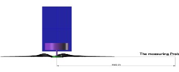
Fig. 9. Anemometer location.
The output power is measured by two avometers. First avometer adjusted and connected series to measured current. The second adjusted and connected parallel to measure the voltage. A flam lamp works a load of the wind turbine, to en- sure pure resistive load (to pass DC current). In field data, the electrical power is measured at same time of wind speed measured, because instantaneous change in voltage and cur- rent. The efficiency of generator is taken in the work as con- stant value about (0.8). As compared, electricity system has efficiency (0.7-0.9) at range of (50-300 rpm of generator shaft speed), Ziter [10].Those make value of electrical power more close to mechanical power been measured.
The Digital Contact Optical Tachometer DT-2236A model ,
measures the wind turbine shaft speed .it use optical configu-
ration, because optical configuration is easy to take reading

and have more accuracy.
Fig. 8. Wind turbine model

IJSER © 2015 http://www.ijser.org

International Journal of Scientific & Engineering Research, Volume 6, Issue 1, January-2015

ISSN 2229-5518

64

3 THEORETICAL ANALYSIS OF CFD

Another technique used to predicate the performance of wind turbine is the Computational Fluid Dynamic (CFD). The CFD involves the numerical solution of the differential gov- erning equations of fluid flows, with the help of computers. This technique has a wide range of engineering applications. In the field of aerodynamic research, this technique has be- come increasingly important and it is prominent for studying turbomachinery.
In commercial codes, a friendly interface gives the user the possibility of easy setting the various options and analyzes the results. Three large parts are generally indicated of a CFD code, which correspond to three phases of the problem analy- sis. As an example ANSYS CFX v13 [11], is used in present study.
The Reynolds’s Averaged Navier-Stokes (RANS) equations for the compressible fluid flow are included the equations of the conservation of mass and momentum. The CFD solver used for the purpose of this work is a k-ε turbulent model. When approaching the study of fluid dynamics problems, the mathematical model is based on the fundamental mass, mo- mentum and energy conservation principles. Therefore, the conservation laws are invoked in the following, in the vectori- al notation and conservative form for unsteady, three– dimensional compressible flow.
Grid generation converts the geometry into a format that can be understood by the CFD solver. It is often the most time consuming and tedious jobs in achieving the CFD solution. Grid generation is the most important before pre-processing step. It is very important to generate accurate grids for the solver to obtain correct results. The accuracy of the CFD solu- tion depends on the quality of the grid used to perform the calculations.
The blade and the whole rotor assembly were modeled us- ing turbo grid. The 3D blade geometry is drawn using Rhinoc- eros 4.0, as shown in Fig. 10. The ANSYS BladeModeler is used to enter CAD file, which include wind turbine blade to turbo grid. It is a part of ANSYS Workbench 13, which able to read CAD file and transfer data reading to grid generation program such as turbo grid. This technique has many ad- vantages, reading shape with high accuracy and save time and labor needing to enter data.


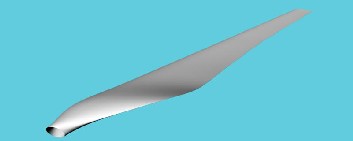
Fig. 10. 3D blade geometry using Rhinoceros 4.0
Turbo grid makes the one passage of flow, which includes one blade and defines the flow region (hub, shroud, inlet and outlet) .Fig. 11 shows the turbo grid passage. It used H/J/C/L- grid to make the flow region and O-grid in close to blade surface. The passage is copied two times with rotating angle 1200 to full complete wind turbine rotor. This passage is defined as rotating section of wind turbine.
The surrounding region of the wind turbine is consist of


Fig. 11. Turbo grid flow passage.
three part one cylinder before the wind turbine, ring outer the turbo grid passage and cylinder after the wind turbine. The grid of this surrounding is made by using mesh tool in ANSYS Workbench v13 as CFX solver reference.
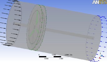
The interface between these two meshes is the GGI inter- face. The outer face of the rotating mesh is the shadow patch of the inner face of the stationary mesh. Fig. 12 shows the GGI patches in the domain. The frozen rotor model is type of GGI interface, which available to use in ANSYS CFX v13.The three frozen rotor interfaces are used in this model .the first one is used between the passage inlet, side of outer ring and surface of the inlet cylinder. The second interface is used between the shroud of passage and the inner surface of the outer ring. The last interface is used between the outer passage, side ring of outer ring, and surface of outlet cylinder.
Velocity inlet and rotational speed of rotating frame are changed in real operation condition. Different values of inlet velocity and rotational speed are entered as boundary condi- tion. Table 1 shows the values of these parameters at many cases. Velocity inlet boundaries have been defined at the up- stream face of the inlet cylinder, shown in Fig. 12 by black ar- row (one head). Opening Pressure outlet boundaries have been defined at the downstream face of the outlet cylinder, shown by blue arrow (two head). Opening pressure outlet is equal to reference pressure of model by adding expression in ANSYS CFX-Pre. Symmetry boundary condition has been assigned to the curved surface of the surrounding domain as wall/slip boundary condition. The rotor faces have been as- signed interface with surrounding domain. The blade has put wall/ no-slip boundary condition.

IJSER © 2015 http://www.ijser.org

International Journal of Scientific & Engineering Research, Volume 6, Issue 1, January-2015

ISSN 2229-5518

65

Fig. 12. Complete grid of wind turbine model to show the GGI interface.

Table 1 Boundray condition table for wind turbine model.

4 RESULTS AND DISCUSSION

4.1 Computational Fluid Dynamic Results

The Computational Fluid Dynamic (CFD) is used to pre- dict the performance of the small wind turbine, as well as, the detailed of the distribution of the different flow parameters. The axil air velocity and, pressure are calculated across the different domains. The wake structure after the wind turbine is also predicted.
The wake is symmetry while the vortices are diffusing in the stream direction as shown in Fig. 13. To get the clearest view of the iso-surface contour, the pressure value is taken as vacuum 0.5 pa (green) that selected by iteration. However, this diffusion of vortices can also be attributed to the grid reso- lution, which becomes coarser towards the outlet.
To illustrate the pressure distribution in all locations , the three sections across the domain along the plane of the wind turbine are shown in Fig. 14.The first contour is taken at 0.75m before the rotor, the second and third contours are taken at
1.5m and 3m respectively after the rotor. The pressure con- tour before rotor shows the effect of the wind turbine blade. The pressure is increasing with the decreasing of the inlet air velocity, which discussed in Actuator disk theory expressed by axial induction factor (a).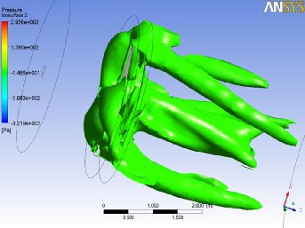


Fig. 13. Iso-surface of -0.5 pa pressure.
Two pressure contours behind the rotor show the wind turbine pressure. The positions of the tip and hub vortices are changed due to the rotation of the wind turbine rotor. The pressure contour far from the rotor is lower than that just be- hind the rotor. Because of the disappearances vortex take place far away of wind turbine.


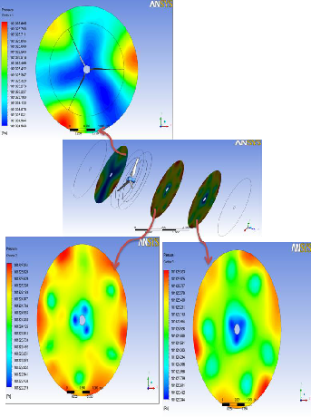
Fig. 14. Pressure contours at different location.

IJSER © 2015 http://www.ijser.org

International Journal of Scientific & Engineering Research, Volume 6, Issue 1, January-2015

ISSN 2229-5518

66

The axial air velocity is calculated at different locations in the three dimensions domain. The upstream and downstream lines of the wind turbine rotor are calculated. The streamlines cross the wind turbine are shown in Fig. 15. As shown from the figure, the tip and root vortex move downstream. The blade tip follows a circular orbit under a free stream axial- directed wind. A trailing vortex of helical path is shed down- stream. The magnitude of velocity distribution around the blades is higher than the others before and after the rotor. Along the blade radius, the magnitude of velocity is increasing from the hub to the tip.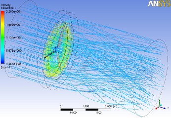


Fig. 15. Stream line cross wind turbine.
Behind the rotor, the shed tip vortices firstly appear as dis- tinct vortex tubes and then merge into a continuous vortex sheet at a short distance from the rotor plane, as shown Figs.
13, 14 and 15. At the blade root, a counter-rotating central vor- tex is shed downstream. Fig. 16 shows the tangential velocity vector at 1m after the rotor that reveals the counter vortex. The root vortex is slower velocity than that of tip. Therefor the tangential velocity gradient is lower than that of the tip be- cause the peripheral velocity increases with the increase of rotor radius. The vorticity field structure follows the classical signature derived from merely theoretical considerations by Carcangiu [12], as shown in Fig. 17.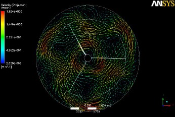


Fig. 16. Tangential velocity vector after rotor.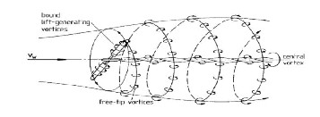


Fig. 17. Theoretical considerations of the vorticity field structure [12].

4.2 Experimental Result

The performance of a wind turbine could be simulated by CFD, however the actual measured performance is needed to validate and confirm the simulation results.The direction of the wind speed is determined to get the maximum axial air velocity. the small turbine is located on a vehicle moving with different constant speeds. The values are selected to be close to the real values of wind speed in Aswan. The electrical voltage and current are measured at different wind speed to get the output power.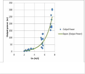

Figure 18 shows Scatter of directly measured power versus wind speed. There are different values of output power at the same wind speed because produced power influence by the wind shear and the turbulence. Overlapping the raw meas- ured data used to obtain the averaged power outputs. At val- ues of the wind speed from 2 to 5 m/s, the output power gradually increases with the increase of wind speed. At values of the wind speed from 5 to 7.5 m/s, the output power sharply increases with the increase of wind speed. Therefore, increas- ing in the wind speed with 33% increases the output power with 87%. The behavior of the output power with the wind speed in the present study is the same as of Song [4]and Ziter [10], who used Vehicle-based system of wind turbine test.
Fig. 18. Scatter of directly measured power versus wind speed.

IJSER © 2015 http://www.ijser.org

International Journal of Scientific & Engineering Research, Volume 6, Issue 1, January-2015

ISSN 2229-5518

67

4. 3 Comparison between the Matlab, CFD and the experimental results

Figure 19 shows the measured and predicted output power with the wind speed. Overlapping the raw measured and cal- culated data used to get the average output power. The meas- ured and calculated powers increase with the increase of wind speed. As shown in the figure, both measured and calculated powers have the same behavior, but the calculated power is greater than the measured.
At the same wind speed, the calculated output power is greater than the measured because the effect of mechanical and electrical losses did not take into account in CFD. The me- chanical loss such as bearing frication is variable with the rota- tional speed of the shaft. Analytical power model calculated the aerodynamic power which absorbed by blade turbine.


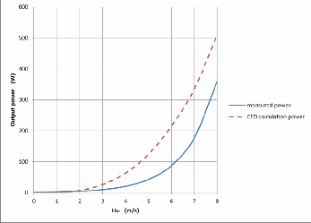
Fig. 19. Comparison between the CFD and the experi- mental results

5 CONCLUSION AND SAMMARY

Using the standard k-ε turbulent model, ANSYS-CFX v13 shows a good agreement with the measured data for a variety of wind speeds (from 0.5 m/s to 5 m/s),as According to the reliable results. The wind turbine power output can be predict- ed under a wider wind speeds range (from 0.5 m/s to 8 m/s), but the accuracy is diminish with increasing the inlet air speed.
Vehicle-based testing was found to be a rapid and effective method for quick evaluation of rotor performance, especially for working wide range of air velocity that not easy found in natu- ral condition. The test results provided sufficient accuracy for evaluation of power performance.
formance predicted by BEM code, because the blade shape con- figuration designed matches the design condition at this range.

NO MENCL ATU RE

a Axial induction factor
a´ Tangential induction factor
A Swept area of a wind turbine rotor
AR Aspect ratio
b Blade span
B Number of blades
c Chord
Cd Drag coefficient
Cl Lift coefficient
dFN Incremental normal force
dFT Incremental tangential force
N Section number p Air pressure
P Wind turbine power output
Q Angular momentum
r Radial position along a wind turbine rotor
Re Reynolds number
Uin Wind speed
Urel Relative wind velocity
X Y, Z Coordinates of axis X, Coordinates of axis Y,
and Coordinates of axis Y
α Angle of attack
ø Angle of relative wind
λ Wind turbine tip speed ratio
λr Local speed ratio
µ Fluid viscosity
θ Pitch angle
θp Section pitch angle
θT Section twist angle
ρ Fluid (air) density
σ Local solidity
ω Angular velocity of the wind
Ω Rotor rotational speed

REF ERENCES

Weather condition of Aswan city was taken as design condi- tion, which considered low in air velocity. The wind turbine have the optimum performance at range 0.5 m/s to 4.5 m/s of air velocity that is revealed by The experimental result and per-

IJSER © 2015 http://www.ijser.org

International Journal of Scientific & Engineering Research, Volume 6, Issue 1, January-2015

ISSN 2229-5518

68

IJSER © 2015 http://www.ijser.org