International Journal of Scientific & Engineering Research Volume 4, Issue 2, February-2013 1
ISSN 2229-5518
Different Modelling and Controlling Technique For
Stabilization Of Inverted Pendulam
K.CHAKRABORTY,,R.R. MUKHERJEE, S. MUKHERJEE
Abstract—In this paper modeling of an inverted pendulum has been done and then two different controllers (PID & SFB) have been used for stabilization of the pendulum. The proposed system extends classical inverted pendulum by incorporating two moving masses. The motion of two masses that slide along the horizontal plane is controllable .The results of computer simulation for the system with Proportional, Integral and Derivative (PID) & State Feedback Controllers are shown.
Index Terms-Inverted pendulam,swing up control,nonlinear control, gain formulae, pole placement,PID controller,State Feedback controller.
1 INTRODUCTION
An inverted pendulum is one of the most commonly studied system in the control area[6]. The control objective of the inverted pendulum is to swing up the pendulum hinged on the moving cart by a linear motor from stable position (vertically down state) to the zero state(vertically upward state) and to keep the pendulum in vertically upward state in spite of the disturbance[1].
In the field of engineering and technology the importance of benchmark[11] needs no explanation. They make it easy to check whether a particular algorithm is giving the requisite results.
A lot of work has been carried out on the inverted pendulum in terms of its stabilization. Many attempts have
been made to control it using classical control ([2],[4]). Thus it is a knowledge which has been widely used in the study of stabilization of space vehicle [6]. It has been used as a test apparatus in computer aided analysis and design thus making it easier to understand and to experiment different control schemes ([3],[5]).
Mathematical models of mechanical systems are usually described by the Newtonion or Euler-Lagrange equations. These models have a structure which is very attractive for the design of control algorithms. This Euler-Lagrange approach has already been proved to be effective in the control design for mechanical and electro –mechanical system [7]. In this paper this method is utilized to investigate global properties of the designed controller.
2. MECHANICAL CONSTRUCTION
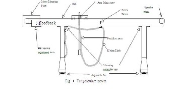
The system comprises of a horizontal plate that is connected to two wheels through a connecting rod. The wheels are independent of each other and are placed in the centre of the rail. Thus the platform can move on a horizontal surface and is able to rotate about the axis of wheels. There are two masses on top of the system that can slide along the horizontal rail, the masses being on both sides of the rail. The system is shown in fig(1)

Kunal Chakraborty is a final year student of M.Tech in the department of Electrical Engineering of Asansol Engineering college Kanyapur, Vivekananda Sarani, Asansol, Burdwan-713305. He received his B.Tech degree in EIE from West Bengal University of Technology in the year 2010. He has two & one number of publications in National & International Conferences.(phone:+91-9563528557,email- sabu_kunal007@yahoo.co.in).He recently joined IMPS Engg. College as Lecturer in EE department.
Rabi Ranjan Mukherjee is a final year student of M.Tech in the department of Electrical Engineering of Asansol Engineering college
Kanyapur, Vivekananda Sarani, Asansol, Burdwan-713305. He received his B.Tech degree in Electrical Engineering from West Bengal University of Technology in the year 2010. He has two & one number of publications in National & International Conferences respectively.(phone:+91-9434664920,email- mukherjee.rabi6@gmail.com)
3 Suvobratra Mukherjee is a final year student of M.Tech in the
department of Electrical Engineering of Asansol Engineering college Kanyapur, Vivekananda Sarani, Asansol, Burdwan-713305. He received his B.Tech degree in Electrical Engineering from West Bengal University of Technology in the year 2007. He is also an Assistant Professor in
Dept. of E.E, IMPS Engineering College, Malda. He has two & oIJnSeER © 2013
3.MATHEMATICAL MODEL OF PHYSICAL SYSTEM :
The inverted pendulum is a classical problem in dynamics and control theory and is widely used as a benchmark for
number of publications in National & Internathiottpn:/a/wl ww.ijser.org
Conferences.(phone:+91-8906128302,email-elec.engg07
@gmail.com)
International Journal of Scientific & Engineering Research Volume 4, Issue 2, February-2013 2
ISSN 2229-5518
testing control algorithms’ (PID controllers, SFB etc). Balancing the cart & pendulum is related to rocket or missile guidance where the centre of gravity is located behind the centre of drag causing aerodynamic instabity.
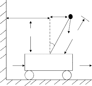
As a more realistic example of the design and simulation of controlled systems we now focus on the development and analysis of an inverted pendulum on a motor driven cart. A sketch of this system is shown in fig(2).
To study the system in detail we need its mathematical model. In this paper we find the mathematical model of the system using Euler-Lagrange’s equations.
The resulting non-linear model is then linearized
Pendulum damping coefficient(D) | 0.005 | Mm/rad |
Moment of inertia of pendulum(L) | 0.099 | Kg/m2 |
Gravitation force(G) | 9.8 | m/s2 |
F= control force; X=displacement of the cart;
8 =pendulum angle from vertical;
Let V1 be the resultant velocity
V1 2 = x 2 + y 2
1 1
The cart with an inverted pendulum, shown below is
bumped with an impulse force F. The dynamic equation of motion for the system is linearized about the pendulum’s
angle, theta. The physical data [9] of the system are given
Therefore kinetic energy of the pendulum,
in table no 1.

K 1mV +
2

1Iw2
2
1 2 2 2 1 2
x1 = x + sin 8
ℓsin8


= m (x +2lx8cos8+ml 8 ] + I8
2 2
Kinetic energy of the of the cart,
1 2

K2 = Mx ,
2
y1 = cos 8
mg
Potential energy of the pendulum, P1 = mglcos8
Potential energy of the cart P2 =0
The Lagrangian of the entire system is given as,
F


L= 1(mx2 +2mlx  cos8+ml282+Mx2)+ I82 ]-mglcos8
M 2 2
The Euler-Lagrange’s equation for the cart &resultant system
X is given as
Fig 2 : The Inverted Pendulum System
d 8L


−
dt 8x
d 8L


−
8L

8x + bx = F
8L

+ d8 = 0
Table 1. Parameters of the system from feedback instrument
.U.K.
dt 88 88
Using these two above equations and putting the system parameters value we get,
( + m 2 )8 + m cos 8 x − m sin 8 + d8 = 0
(M + m)x + m cos 8 8 − m sin 8 82 + bx = F
The above equation shows the dynamics of the system.
IJSER © 2013 http://www.ijser.org
International Journal of Scientific & Engineering Research Volume 4, Issue 2, February-2013 3
ISSN 2229-5518
4. LINEAR DIFFERENTIAL EQUATION MODELING
In order to derive the system transfer functions, we need to liberalize the differtional equation obtained so far. For small angle deviation around equilibrium point .When
pendulum is in upright position sin 8 = 8, cos 8 = 1, 82 = 0
Using above relation we can write as,
X1
Y= 1 0 0 0 X2
0 0 1 0 X3
X4
7. PID Controller design:
The mathematical equation for PID control is
de (t) t
r8+qx-k8+d  =0
=0

ea (t) = Kpe(t) + Kd
dt + Ki e(T) dT
px + q8 + bx = F
Where , (M+m)= p, mgl=k, ml=q, I+ml2=r
5 Transfer Function Modelling:
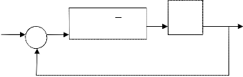
The block diagram of the whole system is shoen in fig (3)
Ki
After taking Laplace transform of linear differential equation we get the following T.F. model,
R(S) + E(s) Kp+sKd + s
-
G(S) C(S)
(s)
-qs2

θ(s)

F(s) = rs2 -k+ ds
−0.2783 S2
Fig3:- Block Diagram of a system with PID Controller
x(s)


F(s) = s (s + 2.026) (s − 1.978) (s + 0.03402)
&
rs2-k+ds
8. State Feedback Controller Design:-
CONDITIONS:


F(s) = (pr-q2)s4 + (pd+br)s3 +(bd-pk)s2-kbs
Our problem is to have a closed loop system having an
overshoot of 10% and settling time of 1 sec. Since the
X(s)
0.68843 (s + 2.014) (s − 1.967)
overshoot


F(s) = s (s + 2.026) (s − 1.978) (s + 0.03402)

MP=e-rr � j1- �
=0.1.
6 State Space Modeling:
Let,8=x1, 8=x2=x1, 8=x2=x1 and, x = x3 , x=x4=x3, x=x4=x3
From state space modeling, the system matrices are found in
vector from given below.
Therefore, ξ = 0.591328 and wn=6.7644 rad/sec. The dominant poles are at=-4 ± j5.45531, the third and fourth pole are placed 5 & 10 times deeper into the s-plane than the dominant poles. Hence the desired characteristics equation:-
s4 + 68s3 +845.7604s2 +9625.6s + 36608.32 =0
A=
0
4.0088
1
−0.047753952
0 0.0000000
0 0.0139155

Let gain, k= [k1 k2 k3 k4]
and
0 0 0 1.0000000
0.116806166 0.0939155 0 0.0344200
0

A – Bk= 0 0 1 0
0 0 0 1
0 0 0 1
−0.27831
B=
0
0.68842
- k1 0.2346-k2 6.8963-k3 -0.0765- k4
Closed loop characteristics equation:-
The output equations are
IJSER © 2013 http://www.ijser.org
International Journal of Scientific & Engineering Research Volume 4, Issue 2, February-2013 4
ISSN 2229-5518
S4 +(0.0765-k4)s3 +(-6.8963 + k3)s2 +(-0.2346 +k2)s +k1 = 0
Comparing all the coefficient of above equation we found.
K = [36608.32 9625.8346 852.6567 -67.9235]
9. Simulation and Results:-.
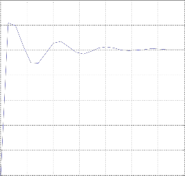
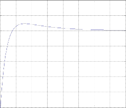
9.1-Stabilisation of position of the cart with PID
controller.
1.4
1.2
1
0.8
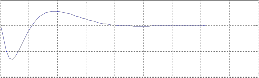
Step Response
1.4
1.2
1
0.8
0.6
Step Res pons e
0.6
0.4
0.2
0
0 2 4 6 8 10 12 14
Time (sec)
0.4
Fig4(c): step response of the system when angle as output for small time
0.2
0
0 0.1 0.2 0.3 0.4 0.5 0.6 0.7 0.8
Time (sec)
1.4
1.2
Step Response
Fig4(a) : step response of the system when position as output for small time
For stabilization we found the PID controller parameters
are,
1
0.8
Kd : - 45 KK : - 200 KK : - 24.2
0.6
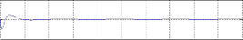
1.4
1.2
1
0.8
Step Respons e
0.4
0.2
0
0 100 200 300 400 500 600 700 800 900 1000
Time (sec)
0.6
0.4
0.2
0
0 100 200 300 400 500 600 700 800 900 1000
Time (sec)
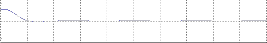
Fig4(b): step response of the system when position as output for large time
9.1.1-Stabilisation of angel of the cart with PID
controller.
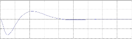
Fig4(d):- step response of the system when angle as output for small time and large time
For stabilization we found the PID controller parameters
are,
KD =-50 kp= -58 Ki = -150
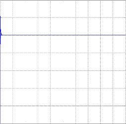
9.2-Stabilisation of Angle of the Pendulum by State
Feedback Controller with Initial Condition:-
IJSER © 2013 http://www.ijser.org
International Journal of Scientific & Engineering Research Volume 4, Issue 2, February-2013 5
ISSN 2229-5518
0.2
0
response due to initial conditions
the system can be stabilized. while PID controller method is cumbersome because of selection of constants of controller, the controller parameters in case of state feedback are chosen analytically. Constant of the controllers can be tuned by some optimization technique
-0.2
0 0.5 1 1.5 2 2.5 3 3.5 4 4.5 5
response due to initial conditions
0.5
0 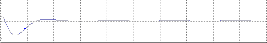
-0.5
0 0.5 1 1.5 2 2.5 3 3.5 4 4.5 5
response due to initial conditions
5
0 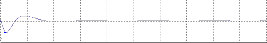
-5
0 0.5 1 1.5 2 2.5 3 3.5 4 4.5 5
response due to initial conditions
for better result.
REFERENCES:
[1]H. J. T Smith, “experimental study on inverted pendulum in April 1992”. IEEE 1991.
[2] Alan Bradshaw and Jindi Shao, “Swing-up control of inverted pendulum systems”, robotica,1996 , volume 14. pp 397-405.
[4] Mario E. Magana and Frank Holzapfel, “Fuzzy –Logic Control of an inverted pendulum with Vision Feedback”, IEEE transactions on education, volume 41, no. 2, May 1998.
100
0
-100
0 0.5 1 1.5 2 2.5 3 3.5 4 4.5 5
[5] K.J. Astrom and K. Furuta, “Swinging up a pendulum by energy control”, Automatic 36 (2000) 287-295, Received 13 November 1997; revised 10
August 1998; received in final form 10 May 1999.
[6] feedback instrument,U.K
Fig5.7:- Response of state feedback controller considering initial condition in
MATLAB
9.2.1-Step Response of the System by State
Feedback Controller:-
[7] I.J.Nagrath, M.Goplal, Control Systems Engineering fourth edition,1975 [8]Ogata,ModernControlEngineering,Fourth Edition,2006
-4
x 10
5
Step Respons e
0
-5
-10
0 0.5 1 1.5 2 2.5 3 3.5 4 4.5
Time (s ec )
-4
x 10
2
Step Respons e
1
0
-1
-2
0 0.2 0.4 0.6 0.8 1 1.2 1.4 1.6 1.8
Time (s ec )
Fig5.8:- Response of Transfer Function represents Angle as output using state feedback controller considering Step input in MATLAB
10. Conclusion:-
Modelling of inverted pendulum shows that system is unstable with non-minimum phase zero. Results of applying two different controllers (PID & SFB) show that
IJSER © 2013 http://www.ijser.org