International Journal of Scientific & Engineering Research, Volume 5, Issue 12, December-2014 419
ISSN 2229-5518
Decision Support Models for Iris Nevus Diagnosis Considering Potential Malignancy Oyebade K. Oyedotun1, Ebenezer O. Olaniyi 2, Abdulkader Helwan3, Adnan Khashman4,
1, 2, 3 Near East University, Lefkosa, via Mersin-10, Turkey
1,2,3 Member, Centre of Innovation for Artificial Intelligence (e-mail: oyebade.oyedotun@yahoo.com, obalolu117@gmail.com,
abdulkader.helwan90@gmail.com)3
4 Founding Director, Centre of Innovation for Artificial Intelligence (CiAi), British University of Nicosia, Girne, Mersin 10, Turkey
(e-mail: adnan.khashman@bun.edu.tr)4
Abstract— Iris nevus is a pigmented growth in the eye, typically found in front of the eye, on the iris or around the pupil. Nevi in themselves are usually benign and harmless but the danger lies in it close developmental association with Iris Melanoma which is malignant and severe secondary glaucoma that require prompt medical attention. The bulk of the problem in combating Iris Melanoma and secondary glaucoma lie in late or undiagnosed Iris Nevi. Furthermore, the somewhat large variances in iris presentation of people considering how race and environmental factor determines the colour of the iris, pupil, and especially close regions surrounding the pupil may make nevi diagnosis difficult. The diagnosis of Iris Nevus is usually achieved by taking images of the eye by a medical expert for examination and then invariably archived as medical history may be used to monitor development of malignancy. Early diagnosis of Iris Nevi and hence medical monitoring reduces the risk of complications that may arise due to malignancy. This paper presents artificial neural network and support vector machine models as decision support in classifying processed medical images of the iris which can significantly raise the confidence of medical diagnosis.
Index Terms— Iris Nevus, Image processing, Artificial Neural Networks , Support Vector Machines.
—————————— ——————————
The iris is the coloured part of the eye. It is made up of two layers. The outer "stroma" can be blue, hazel, green or brown and other back layer (the iris pigment epithelium) is always brown[1].
A tumour is an abnormal mass of tissue which is caused by uncontrolled cellular proliferation and growth. A tumour can either be malignant (cancerous) or benign. A malignant tu- mour is one in which there is rapidly progressive growth with resultant local tissue invasion and distance metastasis. Mean- while, a benign tumour exhibits slowly progressive growth, without local invasion and distance metastasis, but with a po- tential to undergo malignant transformation. Benign tumours are mainly symptomatic due to pressure effect and substances that they elaborate.
Iris nevus and melanomas are the most common primary tumors of the iris, with an incidence ranging from 50-70% of all iris tumors [2].
Iris nevus is a benign tumour of melanocytes in the epithe- lial lining of the iris. It may give rise to symptoms due to pres- sure effect. A nevus at the iridocorneal angle can give rise to secondary angle-closure glaucoma. Also, care must be taken because there is a potential for malignant transformation into a melanoma. A Melanoma, a malignant tumour of melano- cytes, is a difficult cancer to manage and is associated with a poor prognosis. Early diagnosis is very important. This can be achieved by thorough examination of medical history of pa- tients, coupled with routine monitoring of patients being managed for iris nevus. Eye images of patients that have been taken over the years are studied and compared with recent eye images; this helps to determine if there are changes or new growths.
By Kaplan–Meier estimates, iris nevus growth to melano- ma occurred in <1%, 3%, 4%, 8%, and 11% at 1, 5, 10, 15, and
20 years, respectively [3].
More significantly is the need to say that it is impossible for
medical experts to invariably archive eye images of every pa-
tient unless there is a strong reason to do so. One of the main
justifications to making such decisions will be the conviction
as to the presence of iris nevus by a medical expert. This deci-
sion is usually not that of an easy one in view of how patients’
race and environmental factors may affect the colour (blue,
hazel, green or brown) of the iris. Furthermore, the fact that
most iris nevus primarily occur around regions close to the
pupil and may seem to be shadowed or blended into the dif-
fuse colouration of a healthy pupil can lead to wrong diagno-
sis of patients .i.e. classification of eye images as nevus unaf- fected and therefore no or little attention given to such pa- tients (false negative).
Generally, such eye images are ‘manually-visually’ examined by experts for risk factors; though this is a standard practice but then is also not foolproof considering errors prob- ably due to fatigue, eye conditions of an examiner, and almost invisible pigmentation conceded due patients iris colour etc.
This research work introduces an intelligent approach to diagnosis of iris nevus by classifying processed images of the eye. The designed system will be trained, later on fed with images and will hence output the class of the images depend- ing on the presence of iris nevus.
The designed consideration for input images has been that
a thorough examination of eye images of affected and unaf-
fected patients revealed that most iris nevus are located very
close to or at least tend to diffuse away from the pupil.
IJSER © 2014 http://www.ijser.org
International Journal of Scientific & Engineering Research, Volume 5, Issue 12, December-2014 420
ISSN 2229-5518
Hence, more consideration has been given to regions sur- rounding the pupil during the feature extraction process.
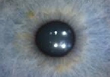
The normal healthy iris has a coloured pupil (usually black or brown), and a distinct clear background or at most the col- our of pupil may diffuse uniformly only very small millimeter away from the pupil and then followed by the clear back- ground as can be seen in fig.1
[4]Fig.1. Iris unaffected with nevus
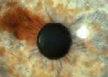
[4]Fig.2. Iris affected with nevus
Conversely, nevi affected irises have coloured pupil as in the healthy case but also some pigments which differ from the colour of the clear background or pupil; at times it invades the iris as non-uniformly distributed shades of the colour of pu- pils as can be seen it fig.2
A feedforward and radial basis function neural networks were designed, trained and used to classify these images. Al- so, support vector machine models were developed to achieve the same task and hence comparison of some crucial perfor- mance parameters presented.
An artificial neural network is a system of simple interconnected computational units called neurons or perceptrons; they are at-
tempts to simulate the structure and function of the brain.
A neural network's ability to perform computations is based on the hope that we can reproduce some of the flexibility and power of the human brain by artificial means [5].
The neurons are connected by links, and each link has a nu- merical weight associated with it. Weights are the basic means of long-term memory in ANNs [6].
The typical convectional Von Neumann’s computer is obvi-
ously faster and more accurate at computing arithmetic but lacks flexibility, noise tolerance; and cannot invariably handle incom- plete data. Most significant is the inability to upgrade its perfor- mance over time from experience. i.e. incapable of learning.
Neural networks on the other hand possess inherent learning capability and its performance can be so designed to improve over time due experiential knowledge.
The processing unit or element of the neuron works to sum up the product of the inputs and corresponding weights, the result is known as total potential(T.P).
The rule used to determine neuron activation is given below
[7].
T.P ≥ Threshold: Neuron fires or activates
T.P < Threshold: Neuron does not fire or activate
Where threshold is a reference value to which the T.P is compared.
Neural networks usually have an input layer, an output layer and optional hidden layer(s); also, the number of neurons at each layer may vary depending on design and problem to be solved. Neural networks with hidden layers are known as multilayer net- works and are very useful when computing linearly inseparable data.
Multilayer neural networks bear applications in pattern recog- nition, regression problems, data mining etc.
The phase of building knowledge into neural networks is called learning or training. The three basic types of learning par- adigms are:
-Supervised learning: the network is given examples and con- currently supplied the desired outputs; the network is generally meant to minimize a cost function in order to achieve this, usual- ly an accumulated error between desired outputs and the actual outputs.
Error per training pattern = desired output - actual output
Accumulated error= ∑(error of training patterns)
-Unsupervised learning: the network is given examples but not supplied with the corresponding outputs; the network is meant to determine patterns between the inputs attributes (examples) ac- cording to some criteria and therefore group the examples thus.
-Reinforced learning: there is no desired output present into the data set but there is a positive or negative feedback depending on output (desired/undesired) [8].
The most common multilayer neural network used is the feed- forward network; they work on supervised learning algorithms and are also known as backpropagation networks considering how learning is achieved. i.e. errors accumulated at the output layer are propagated back into the network for the adjustment of weights. It is noted that there is no backward pass of computation of any such except during training. i.e. all links proceed in the forward direction during simulation.
IJSER © 2014 http://www.ijser.org
International Journal of Scientific & Engineering Research, Volume 5, Issue 12, December-2014 421
ISSN 2229-5518
Fig.3. Feedforward neural network
Each input neuron takes a value of the input pattern or vector attributes, therefore the number of input neurons will be number of attributes or elements that describe the input patterns. The number of hidden of neurons is usually obtained heuristically during the training phase; and the number of output neurons equals the number of different categories in dataset for classification problems.
Backpropagation algorithm is based and which is used to up- date weights of feedforward networks is shown below [9].
1. Initial weights and thresholds to small random numbers.
2. Randomly choose an input pattern x(u)
3. Propagate the signal forward through the network
4. Compute δiL in the output layer (oi = yi L)
Radial basis function networks are very similar to the back- propagation networks in architecture; the fundamental difference being in the analogy behind weight computation, the activation function used at the neurons’ outputs, and that they basically have one hidden layer .
In the context of a neural network, the hidden units provide a set of “functions” that constitute arbitrarily the “basis” for input patterns when they are expanded into hidden space; these func- tions are called radial-basis functions[10].
The motivation behind RBFN and some other neural classifiers is based on the knowledge that pattern transformed to a higher- dimensional space which is nonlinear is more probable to be line- arly separable than in the low-dimensional vector representations of the same patterns (covers’s separability theorem on patterns). The output of neuron units are calculated using k-means clustering similar algorithms, after which Gaussian function is applied to provide the unit final output. During training, the hidden layer neurons are centered usually randomly in space on subsets or all of the training patterns space (dimensionality is of the training pattern) [11]; after which the Euclidean distance between each neuron and training pattern vectors are calculated, then the radial basis function (also or referred to as a kernel) applied to calculated distances.
The radial basis function is so named because the radius distance is the argument to the function [12].
Weight = RBFN (dis tan ce)
It is to be noted that while other functions such as logistic and thin-plate spline can be used in RBFN networks, the Gaussian functions is the most common. During training, the radius of Gaussian function is usually chosen; and this affects the extent to
δ L = g ' (h L )[d L − y L ]
(1)
which neurons have influence considering distance.
i i i i
Where h iL represents the net input to the ith unit in the lth layer, and g’ is the derivative of the activation function g.
5. Compute the deltas for the preceding layers by propagat- ing the error backwards.
The best predicted value for the new point is found by sum- ming the output values of the RBF functions multiplied by weights computed for each neuron[12].
The equation relating Gaussian function output to the distance from data points (r>0) to neurons centre is given below.
− r 2
l = l ∑
l +1
l +1
δ i g ' (hi )
j
wij δ j
(2)![]()
Φ(r ) = e 2σ
(4)
For l = (L-1),…….,1.
6. Update weights using
Where, σ is used to control the smoothness of the interpolating function [11]; and r is the Euclidean distance from a neuron center
∆ l =
l l −1
to a training data point.
wij
ηδ i y j
(3)
7. Go to step 2 and repeat for the next pattern until error in
the output layer is below the pre-specified threshold or maximum number of iterations is reached.
Where wj are weights connected to neuron j, xj are input pat- terns, d is the desired output, y is the actual output, t is iteration number, and η (0.0< η <1.0) is the learning rate or step size [9].
Usually, another term known as momentum, α (0.0< α<1.0), is at times included in equation 1 so that the risk of error gradient minimization getting stuck in a local minimum is significantly reduced.
They are basically classifiers which work on maximum margin algorithm to create the optimal decision surface. They are very power and useful in categorization problems; some regression version of the algorithm also exists. They give very impressive performance on generalization even with the fact they usually lack domain-specific knowledge input.
A notion that is central to support vector learning algorithm is the inner-product kernel between a support vector xi and the vector x drawn from input space. Support Vectors are the ex-
IJSER © 2014 http://www.ijser.org
International Journal of Scientific & Engineering Research, Volume 5, Issue 12, December-2014 422
ISSN 2229-5518
amples closest to the separating hyperplane and the aim of SVMs is to orientate this hyperplane in such a way as to be as far as possible from the closest members of both classes [13].
The most significant attribute of SVMs is the confidence that the resulting decision hyperplane is optimal (provides the maxi- mum margin of separation between different classes), in contrast to neural networks that occasionally get stuck in local minima;
besides neural networks invariably converges to different or at
least slightly different solutions each time they are re-initialized for training.
What the maximum margin algorithm does is using some con- straints select some points from the training data, these points only are then used to determine the position and orientation of the deci-
sion hyperplane; all other points are of no consequence.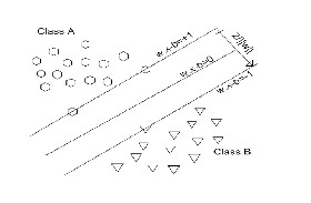
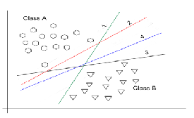
Fig.4. Support vector machine
It is assumed that for a training dataset containing two classes denoted as hexagons and triangles, the maximum margin algo- rithm extracts support vectors from each class contained in the training dataset. i.e. equations are below
Fig.5. Different obtainable hyperplanes for a two-class data classi- fication
The aim of this research is design intelligent models such that when supplied eye images, outputs their corresponding classes depending on whether nevus is present or absent.
The images are first processed to extract features or patterns of interest that the designed models are meant to learn.
The motivation behind the input design is such that after com- prehensive study of nevus affected and unaffected eye images, it was observed that regions close to the pupil are mostly always the affected, hence not the whole iris images were used but an area extending only some few millimeters from the pupil were extract- ed for processing.
Furthermore, it was observed that for unaffected irises, the pu- pil colour (usually black or brown) is distinct compared to the rest of the iris background or only diffuses gradually and uniformly blends into the background (iris). In contrast, the colour of pig- mentation could be different from the colour of the iris, or when
Class A, two hexagons on line: w . x i + b = + 1
Class B, one triangle on line w . x i + b = - 1
(5) (6)
it’s even the same as the pupil, diffusion from the pupil contrast quite significantly with the iris or strikingly non-uniform.
The decision hyperplane is the centre of space between the margin, and its equation is given as
Hence, the images have been processed as shown below.
• Rotation: images were rotated 15º incrementally through
w . x i + b = 0
The margin width is obtained as M = 2/ || w ||
(7)
(8)
to 360º
• Conversion from colour to grayscale
The final goal of the algorithm is to maximize M, which is in turn achieved by minimizing w through sequential minimal optimiza- tion, quadratic programming or least squares then carrying out some constraint computations using Lagrange multipliers.
In fig.5, some different obtainable hyperplanes when classifying data are shown. It is noteworthy that a neural network could ran- domly arrive at any of the decision planes for each different train- ing, even with the same learning parameters.i.e. Fig.5. (lines 1 to
4).
In contrast, support vector machines will after training converge to the hyperplane with maximum margin between the two classes.i.e. fig.5. (blue line 4)
• Filtering: 10×20 mask median filter
• Rescaling: images rescaled to 30×30 pixels using pattern averaging.
• Normalization: pixel values were normalized to values from 0 & 1 range.
• Reshaping: each input image was reshaped to 900×1.
Rotational invariance was built into the designed models by ro- tating training images 15º incrementally through to 360º, as this makes the systems more robust and the significantly enhances the capability of such designed models to capture classification re- gardless of image orientation.
The median filter has been used to amplify the significance
of contrast in situations where the pupil colour tends to diffuse into the iris.i.e. when it diffuses gradually, the median filter makes it more gradual and when it diffuses sharply, the median filter
IJSER © 2014 http://www.ijser.org
International Journal of Scientific & Engineering Research, Volume 5, Issue 12, December-2014 423
ISSN 2229-5518
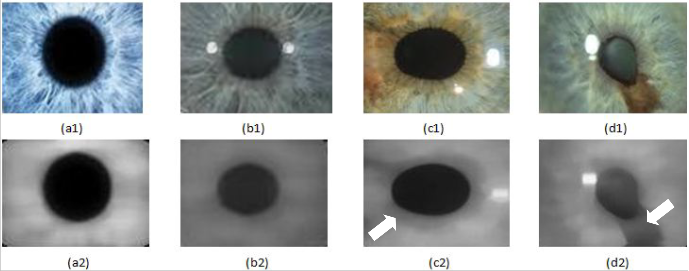
[4]Fig.6. Images of nevi unaffected and affected irises (white arrows showing affected regions)
magnifies the sharpness. Also, it helps removed reflection of camera screen that appears on the images.
The images were then rescaled to 30×30 pixels (900pixels) to ease computation, using pattern averaging.
Below in Fig.6 is shown some of processed images used for training the designed models.
Original colour images of irises that are unaffected with nevus in are shown fig.6. (a1) & (b2), while their processed images are shown directly below them correspondingly. i.e. (a2) & (b2). Al- so, original colour images of affected irises are shown in fig.6. (c1) & (d1), while their processed images are shown directly be- low them correspondingly as (c2) & (d2).
Since there are only two classes of output, it then follows that out- put coding for nevus classification using the neural network mod- els was achieved as shown below.
Nevus unaffected iris: [0 1] Nevus affected iris: [1 0]
For the SVM model, output coding is shown below. Nevus unaffected iris: class 1
Nevus affected iris: class 2
The input images for training the designed models are of
900pixels each, therefore, BPNN model has 900 input neurons.
Also, since there two classes of the output, the network has two output neurons.
The network was trained with 500 samples of iris images con- taining both classes of interest.
The training of the BPNN model was achieved using various learning parameters such as number of hidden neurons, learning rate, momentum rate, maximum epochs; but the parameters which achieved best performance are shown in table 1.
The number of neurons at the hidden layer was heuristically obtained as 35.
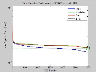
The plot in Fig.7. shows the Mean Square Error (MSE) plotted against the number of epochs. Also, the blue, green and red lines represent the training, validation and test curves respectively. MATLAB software and programming have been used to achieve the learning; where a default 15% of the training data has been used as validation set to avoid over-fitting of the trained model. Hence, during training, validation occurs concurrently and when even error on the training data is stilling but the error on the vali- dation set starts to increase, training is stopped to avoid the net- work memorizing data.
It will therefore be seen in fig.7. that training was stopped only some epochs away from when network tends to begin to over- fitting and more significantly is that network performance is clipped considering the MSE on the validation set (broken straight line in fig.7.).
The test curve lies almost directly on the validation curve showing its MSE follows that of the validation set.i.e. double checking network performance during training.
IJSER © 2014 http://www.ijser.org
International Journal of Scientific & Engineering Research, Volume 5, Issue 12, December-2014 424
ISSN 2229-5518
Since the architecture of a RBFN and BPNN are almost basically the same but for the way weights are updated and activations functions used; therefore, the number of input and output neurons remains the same while the number of hidden neurons was heuris- tically obtained during training as 200.
The MSE plot for the network is shown fig.7. and network training parameters shown is table 3.
The MSE performance goal of the RBFN was set to 0.02 be- fore the commencement of training, a Gaussian function was cho- sen as neurons squashing function and spread constant of 2 was used.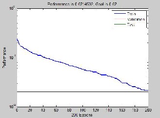
Fig.7. MSE plot of BPNN training.
Table 1: Heuristic BPNN training network parameters
Fig.8. MSE plot of RBFN training.
Table 3: Heuristic RBFN training network parameters
The trained network has been tested using 316 iris images
(38.7% of whole data) and obtained performance is shown in table
2.
Table 2: BPNN network test performance
Network test performance is shown below; the same number of test used on the BPPN model was also used here.
It is to be noted that any of the test data were not part of the training set.
IJSER © 2014 http://www.ijser.org
International Journal of Scientific & Engineering Research, Volume 5, Issue 12, December-2014 425
ISSN 2229-5518
Table 4: RBFN network test performance
Table 6: SVM quadratic kernel model training & test per- formance
The RBFN model was simulated too with the same test data used on the BPNN and result shown above.
The SVM model was also trained using MATLAB software, using
500 training samples and 300 test samples. i.e. same that
was used in the earlier neural network models.
A default 10% cross-validation has also been used here to
avoid model over-fitting training data and hence losing gener- alization power.
During training, it was observed that model had problems con-
verging to a solution within the default maximum epochs of
15,000; hence the number of maximum epochs was increased to
30,000 to allow for convergence.
Also, two SVM model were trained; one using a liner kernel and the other using a quadratic kernel.
The training parameters and test performance using the linear kernel is shown in table 5.
Table 5: SVM linear kernel model training & test performance
The performance analysis of various models designed to classify nevus affected and unaffected iris images is presented in the table below. It is to be noted that the SVM model (using quadratic ker- nel) with the better test performance has been used in the compar- ison analysis against BPNN and RBFN neural network models. Note that N/A means Not Applicable.
Table 7: Comparative analysis of models performances
Number of training samples | 500 |
Number of support vectors | 307 |
Kernel function | linear |
K-fold cross validation | 10 |
Maximum epochs | >15,000 |
Number of test samples | 316 |
Correctly classified test samples | 229 |
Recognition rate | 72.5% |
The training and test performance for SVM using a quadratic kernel is shown in table 6.
It will be seen from the above table that SVM outperforms both neural network models in terms of recognition rates. This can be attributed to the motivation behind the learning algorithm form SVM which constraints the decision boundary to converge at sep- aration of maximum margin between the two classes of output.
IJSER © 2014 http://www.ijser.org
International Journal of Scientific & Engineering Research, Volume 5, Issue 12, December-2014 426
ISSN 2229-5518
Also, the training time for SVM is the least compared to both neu- ral network models, although required more epochs to converge at the solution.
Both neural network models show no significant differences in terms of training time and recognition rate, but for larger number of hidden neurons required by the RBFN model and conversely larger epochs required by the BPNN to achieve obtained perfor- mance.
This work presents decision support diagnostic models for iris nevus, a benign tumor of the iris. Although an outstanding 90.8% was achieved in one of the models; this research application may not necessarily be a replacement for a medical expert but to a large extent should be very useful in increasing the reliance of expert’s findings on diagnosis.
The tumor occasionally is not a threat to patients but its develop- ment into iris melanoma which is cancerous; or the risk of trans- formation to secondary glaucoma exists in nevus affected patients and are of very serious medical concern often requiring urgent attention.
I wish to specially thank Dr. Tam B. Opusunju of the Safeway specialist hospital, Lagos, for his sound technical reviews, medi- cally, and immense contribution to the introduction section.
[1] The Eye Cancer Foundation Eye Cancer Network Education and Sup- port for Eye Tumor Patients and Their Fami- lies,available:http://www.eyecancer.com/conditions/34/iris- melanoma
[2] Author: Nadia K Waheed, MD, MPH; Chief Editor: Hampton Roy Sr, MD, Iris Melanoma available: http://emedicine.medscape.com/article/1208624-overview
[3] Iris Nevus Growth into Melanoma: Analysis of 1611 Consecutive Eyes, Ocular Oncology Service, Wills Eye Institute, Thomas Jefferson Univer- sity, Philadelphia, Pennsylvania, available: http://www.aaojournal.org/article/S01616420%2812%2900954-2/pdf
[4] The Eye Cancer Foundation, Eye Cancer Network, available:
http://www.eyecancer.com/research/image-gallery/12/iris-tumors
[5] J. Zurada, 1992. Introduction to Artificial Neural Systems, West Publish- ing Company. pp. 2.
[6] Michael Negnevitsky, 2005. Artificial Intelligence: A Guide to Intelligent
Systems, Second Edition. pp.167
[7] Oyebade Oyedotun, Adnan Khashman. Intelligent Road Traffic Control using Artificial Neural Network, Proceedings of 2014 3rd International Conference on Information and Intelligent Computing, Hong Kong.
2014. pp.1.
[8] R. M. Hristev, 1998. The ANN book, GNU Public License, ver. 2, Edition
1. pp.112.
[9] Ani1 K. Jain, Michigan State University, Jianchang Mao, K.M.
Mohiuddin, IBM Almaden Research Center, Artificial Neural Network: A Tutorial. pp.37.
[10] S. Haykins, 1999. Neural Networks: A Comprehensive Foundation, Pren-
tice-Hall International Inc., Second Edition, pp. 256,318.
[11] Ke-Lin Du, M.N.S Swarmy, 2014. Neural Networks and Statistical learn- ing, Springer-Verlag London. pp.303.
[12] RBF Networks, available: http://www.dtreg.com/rbf.htm
[13] T. Fletcher, 2009. Support Vector Machines Explained, University Col-
lege London, pp. 2. , available: www.cs.ucl.ac.uk/staff/T.Fletcher/
————————————————
• O. Oyedotun is a member of Centre of Innovation for Artificial Intelligence, British University of Nicosia, Girne, via Mersin-10, Turkey and currently pur- suing masters degree program in Electrical/Electronic Engineering in Near East University, Lefkosa,via Mersin-10, Turkey. Research interests include artificial neural networks, pattern recognition, machine learning, image processing, fuzzy systems and robotics. PH-+905428892591.
E-mail: oyebade.oyedotun@yahoo.com
• E. Olaniyi is a member of Centre of Innovation for Artificial Intelligence,British University of Nicosia,Girne,via Mersin 10,Turkey.He is also a current master degree student of Electrical/Electronic Engineering in Near East Universi- ty,Lefkosa,via Mersin 10,Turkey.His research interests area are:Artificial neural network,Image processing,speech processing and renewable energy system.
PH- +905428827442. E-mail: obalolu117@yahoo.com
• A. Helwen is a member of the Tissue Engineering and Biomaterials Research Center, Near East University, Nicosia, Mersin-10, Turkey. He is currently studying masters’ degree program in biomedical engineering in Near East Uni- versity. He received his bachelor of engineering in biomedical engineering from Al Manar University of Tripoli, Lebanon, 2013. Research interests include arti- ficial intelligence in medicine, artificial neural networks, image processing, and tissue engineering. E-mail: abdulkader.helwan90@gmail.com
• A. Khashman received B.Eng. degree in electronic and communication engineer- ing from University of Birmingham, England, UK, in 1991, and the M.S and Ph.D. degrees in electronic engineering from University of Nottingham, Eng- land, UK, in 1992 and 1997. During 1998-2001 he was an Assistant Professor and the Chairman of Computer Engineering Department, Near East University, Lefkosa, Turkey. During 2001-2009 he was an Associate Professor and Chair- man of Electrical and Electronic Engineering Department, and in 2009 he re- ceived the professorship. In 2001 he established the Intelligent Systems Research Group (ISRG) at the same university, and has been chairing ISRG until present. From 2007 until 2008 he was also the Vice-Dean of Engineering Faculty, later
on from 2013 until 2014 the Dean of the faculty at the same university. Since
2014, Professor Khashman was appointed as the Founding Dean of Engineering
Faculty at the British University of Nicosia in N. Cyprus, where he also estab- lished the Centre of Innovation for Artificial Intelligence His current research
IJSER © 2014 http://www.ijser.org