International Journal of Scientific & Engineering Research, Volume 6, Issue 4, April-2015 1270
ISSN 2229-5518
DIGITAL IMAGE RESTORATION
Siddaraju K. 1, Gururaju 2
1. Research Scholar and Assistant. Professor of Computer Science, .Maharani’s Science College for
Women, Mysore-570005, Karnataka, India
2. Research Scholar, Department of computer Science
Abstract- Images may be degraded for many reasons for example, out-of-focus optics produce blurred images, and variations in electronic imaging components introduce noise. Reducing blur or noise or both in images is known as image restoration. Multi-channel blind image restoration recovers an original image from several blurred versions without any knowledge of the blur function. In many applications the image to be processed has a multi-channel nature; i.e., there are several image planes available, called channels with redundant as well as complementary information. Here we propose a multichannel blind restoration technique for linearly degraded images without the explicit knowledge of either the Point Spread Function (PSF) or the original image. The blurred noisy image is compressed using 8 by 8 blocks DCT and filtered using zonal filter.
The proposed restoration involves a DCT domain zonal filtering pre-processing followed by a post-processing step of time domain deconvolution. The technique applies to situations on which the scene consists of a finite support object against a uniformly black, gray or white and color backgrounds. Preliminary simulations in noise-free and noisy cases are conducted. The results are compared with standard Median filter for image denoising and the proposed blind restoration scheme is shown to exhibit improvement in SNR.
—————————— ——————————
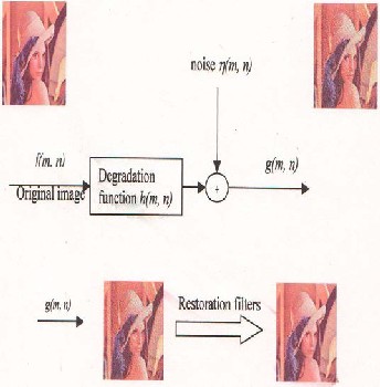
Digital Image restoration attempts to reconstruct or recover an image that has been degrading using a prior knowledge of the degradation phenomenon.
The purpose of image restoration is to “compensate for” “or undo” defects which degrade an image. Degradation comes in many forms such as motion blur, noise, and camera misfocus. In cases like motion blur, it is possible to come up with a very good estimate of the actual blurring function and “undo” the blur to restore the original image. In cases where he image is corrupted by noise, the best we may hope to do is to compensate for the degradation it caused. Restoration techniques are oriented towards modeling the degradation and applying the inverse process in order to recover the original image.
(a)
IJSER © 2015 http://www.ijser.org
International Journal of Scientific & Engineering Research, Volume 6, Issue 4, April-2015 1271
ISSN 2229-5518
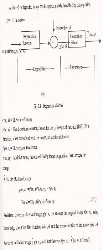
In general the degradation model can be written as:
The blurring or degradation of an image can be caused by many factors:
• Movements during the image capture process, by the camera or, when long exposure times are used, by the subject.
• Out-of-focus optics, use of a wide-angle lens, atmospheric turbulence, or a short exposure time, which reduced the number of photons captured.
• Scattered light distortion in confocal microscopy
There are three principal ways to estimate the degradation function for use in image restoration:
• Observation
• Experimentation
• Mathematical modeling
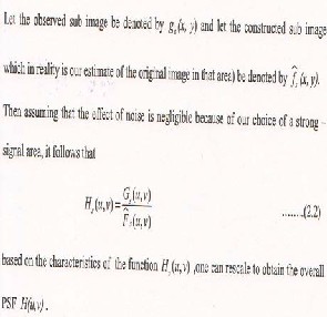
Suppose we are given a degraded image without any knowledge about the degradation function H. One way to estimate this function is to gather information from the image itself. For example if the image is blurred, we can look at a small section of the image containing simple structures, like part of an object and the background. In order to reduce the effect of noise in our observation, we would look for areas of strong signal content. Using sample gray levels of the object and the background, we can construct an unblurred image of the same size and
characteristics as the observed sub image.
IJSER © 2015 http://www.ijser.org
International Journal of Scientific & Engineering Research, Volume 6, Issue 4, April-2015 1272
ISSN 2229-5518
![]() …………….…..… (2.4) Where K is a constant that depends on the nature
…………….…..… (2.4) Where K is a constant that depends on the nature
of the turbulence.
Note that this is similar to a Gaussian low pass filter. Gaussian low pass filter is also often used to model mild uniform blurring.
If equipment similar to that used to acquire the degraded image is available, it is possible to obtain an accurate estimate of the degradation. Images similar to the degraded image can be acquired with various system settings until they are degraded as closely as possible to the image we wish to restore. Then the idea is to obtain the impulse response of the degradation by imaging an impulse (small doe of light) using the same system settings.
An impulse is simulated by a bright dot of light as bright as possible to reduce the effect of noise. Then recalling that the Fourier transform of an impulse is constant, it follows that
![]() ………………… (2.3)
………………… (2.3)
A is the intensity of light source and G(u, v) is the observed Spectrum.
A physical model is often used to obtain
In many situations, the point-spread function h (x, y) is known explicitly prior to the image restoration process. In these cases, the recovery of f(x, y) is known as the classical linear image restoration problem. This problem has been thoroughly studied and a long list of restoration methods for this situation includes numerous well- known techniques, such as inverse filtering, Wiener filtering, least-squares filtering, etc.
In image restoration the goal is to recover an image that has been corrupted or degraded. The more information we have of the degradation process, the better off we are. This is known as a priori knowledge. There are several techniques in image restoration, some use frequency domain concepts; others attempt to model the degradation and apply the inverse process. The modeling approach requires determining a criterion of “goodness” that will yield an “optimal” solution. Using inverse filter we demonstrate the simplest concept in image restoration when the actual spatial convolution filter used to degrade the image is known. Shown below is the blurred image that is the result of convolving a Gaussian filter in the width direction with the original image. This effect is similar to the one observed when a photograph is taken with a camera in motion.
the PSF.
Blurring due to atmospheric turbulence can be modeled by the transfer function:
IJSER © 2015 http://www.ijser.org
International Journal of Scientific & Engineering Research, Volume 6, Issue 4, April-2015 1273
ISSN 2229-5518
f(u, v) is the original image.
The inverse filtering process is them
F(u, v) = G(u, v) / H(u, v)
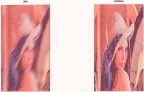
(a) (b)
Fig 2: Inverse Filter Restoration results where a is the Blurred image and b is the restored image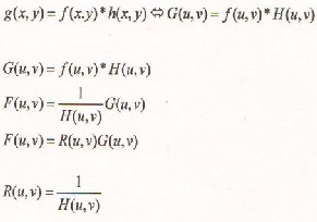
Let f be the original image, h the blurring kernel, and g the blurred image. The idea in inverse filtering is to recover the original image from the blurred image. From the convolution theorem, the DFT of the blurred image is the product of the DFT of the original image and the DFT of the blurring kernel. Thus, dividing the DFT of the blurred image by the DFT of the kernel, we can recover the original image. Then the inverse frequency filter, R(u), to be applied is 1/H(u). We are assuming no noise is present in the system. Observe the difficulties we encounter when H(u) is very small or equal to zero.
………………. (2.5) Where
G(u, v) is the degraded image,
H(u, v) is the degradation transfer function, and
We can see that inverse filtering is a very easy and accurate way to restore an image provided that we know what the blurring filter is and that we have no noise. Because an inverse filter is a high pass filter, it will tend to amplify noise as was presented in our results. The second way of inverse filtering was through an iterative procedure. Since that is more or less an averaging method, it deals a little better with noise by averaging it out. But both methods do not deal well with noise. We must use some method of restoration, which would trade off inverse filtering with de-noising.
There is a technique known as Wiener filtering that is used in image restoration. This technique assumes that if noise is present in the system, then it is considered to be additive white Gaussian noise (AWGN). Wiener filtering normally requires a priori knowledge of the power spectra of the noise and the original image. What if the spectral density functions of the image and noise are unknown? In this case, we use a parametric version of the Wiener filter.
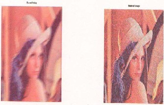
(a) (b) Fig 3: Wiener Filter Restoration results where a is
the Blurred Noisy image (SNR=20dB) and b is the restored image with (MSF=440.PSNR=21.68)
IJSER © 2015 http://www.ijser.org
International Journal of Scientific & Engineering Research, Volume 6, Issue 4, April-2015 1274
ISSN 2229-5518
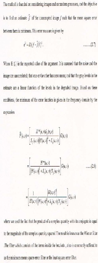
The term in the equation of 8 is as follows: H(u, v)=degradation function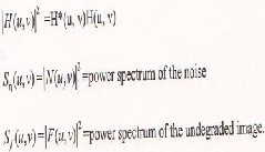
H*(u, v)=complex conjugate of H(u, v)
…… (2.9) H(u, v) is the transform of the degraded function
and g(u, v) is the transform of the degraded image. If the noise is zero, then the noise power spectrum vanishes and the wiener filter reduces to the inverse filter. When we are dealing with spectrally white noise, the spectrum /N(u, v)/2 is a constant, which simplifies things considerably. However the power spectrum of the original image is seldom is known. An approach used frequently when these quantities are not known or cannot be estimated is to approximate equation 7 by the expression
Where K is a specified constant.
The Lucy-Richardson algorithm can be used effectively when the point-spread function PSF (blurring operator) is known, but little or no information is available for the noise. The blurred and noisy image is restored by the iterative, accelerated, damped Lucy-Richardson algorithm. The additional optical system (e.g.camera) Characteristics can be used as input parameters to improve the quality of the image restoration. Simulate a real-life image that could be blurred (e.g., due to camera motion or lack of focus) and noisy (e.g., due to random disturbances). The example simulates the blur by convolving a motion filter with the true image (using imfilter). The motion filter then represents a point-spread function, PSF.
IJSER © 2015 http://www.ijser.org
International Journal of Scientific & Engineering Research, Volume 6, Issue 4, April-2015 1275
ISSN 2229-5518

about the image to be restored, and it is difficult to calculate or measure PSF explicitly. The problem of simultaneously estimating the PSF and restoring an unknown image is called Blind deconvolution.
(a) (b)
Fig 4: Lucy Richardson results where a is the Blurred Noisy image with SNR _20dB, b is Restored image with (MSE=440, PSNR=21.678, Numlt=20)
Deconvolution is a signal-processing operation that unravels the effects of convolution performed by a linear time-invariant system operating on an input image. Degradation are modeled as being the results of convolution, and restoration seeks to find the filters that apply the process in reverse, the filters used in the restoration process often are called deconvolution filters.
An observed image g(x, y) can be described as a convolution of the object brightness distribution f(x, y) by a PSF h(x, y) accounting for the acquisition chain and transfer medium
g(x, y) =h(x, y)*f(x, y) G(u, v) = H(u, v) F(u. v)
in order to recover the object brightness distribution f(x, y), the usual procedure consists in deconvolving g(x, y), but this requires the knowledge of the PSF h(x, y), when no reliable measurement of h(x, y) is available, one can wonder whether it is possible to obtain both f(x, y) and h(x, y) given their convolution product g(x, y). This problem is known as blind deconvolution. In application such as artificial satellite imaging, remote sensing, and medical imaging, improved image quality is often costly or physically
impossible to obtain. In addition little is known
Restoration in the case of known blur, assuming the linear degradation model, is called linear image restoration. In many practical situations, however, the blur is unknown. Hence, both the blur identification and image restoration must be performed from the degraded image. Restoration in the case of unknown blur is called blind image restoration (deconvolution).
However, there are numerous situations in which the point-spread function is not explicitly known, and the true image f(x, y) must be identified directly from the observed image g(x, y) by using partial or no information about the true image and the point-spread function. In these cases, we have the more difficult problem of blind deconvolution. Several methods have been proposed for blind deconvolution and active research continues in this area. In our project, we seek to understand and implement one of the proposed algorithms of blind deconvolution: The iterative blind deconvolution algorithm.
The goal of the general blind deconvolution problem is to recover two convolved signals, f and h, when only a noisy version of their convolution is available along with some or no partial information about either signal. Some important characteristics of the problem of blind deconvolution is listed below:
The true image and the point-spread function must be irreducible for a unique solution to the problem. A signal is reducible if it can be expressed as the convolution of two other signals (neither of which is the two-dimensional delta function). If either the true image or the point- spread function is reducible, then there exists more than one way to perform the deconvolution.
IJSER © 2015 http://www.ijser.org
International Journal of Scientific & Engineering Research, Volume 6, Issue 4, April-2015 1276
ISSN 2229-5518
• Without the use of appropriate a priori information, only a scaled, shifted version of the original image can be obtained through blind deconvolution.
• In the presence of additive noise, the exact blind deconvolution of the observed image g(x,y) is impossible and only an approximate solution can be found.
In practice, all deconvolution algorithms require some partial information to be known and some conditions to be satisfied. The iterative blind deconvolution algorithm is one of the most general algorithms with the least amount of required a priori information. The method requires the true image and the point-spread function to be nonnegative with known finite support. These requirements are not overly constricting since image intensity is always nonnegative and support information can often be inferred in many image- processing situations.
Ayers and Dainty first proposed the iterative blind deconvolution algorithm in 1988. It is one of the most popular and most famous algorithms in blind deconvolution. The basic structure of the algorithm is a simple iterative one and is illustrated in the figure below.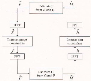
Fig 5: Iterative Blind Deconvolution Algorithm
Starting with a random initial guess for the true image, the algorithm alternates between the image and Fourier domains, using known constraints in each domain. The image domain constrains are simply those imposed by the no negativity requirement and the known finite support information. Negative-valued pixels and nonzero pixels outside the region of support are set to zero. The Fourier domain constraint is a consequence of the fact that if the noise level is low, then the product of the Fourier transforms of the true image and the point-spread function should be approximately equal to the Fourier transform of the observed image. Using this fact, we can use inverse filtering to estimate of the point-spread function (image) using the Fourier transforms of the degraded observation and the estimate of the true image (point-spread function). However, inverse filtering can result in the magnification of noise in regions where the function being inverted has low values. There are several different ways to deal with this problem. In our experiments, we found that the best performance is achieved when the following formula is used to generate a new estimate of H at the k-th iteration:
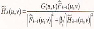 ……..….. (2.11) The formula for generating a new estimate of F is similar. The above formula resembles the Wiener filtering formula and it has the similar effect to providing robustness against noise. The constant beta represents the energy in the additive noise and must be chosen carefully for the algorithm to perform well.
The iterative deconvolution procedure follows a series of steps to calculate its result.
• First, the algorithm guesses what the object looks like.
• Second, the guess is mathematically blurred to simulate the effects of the micro scope’s limited aperture.
IJSER © 2015 http://www.ijser.org
International Journal of Scientific & Engineering Research, Volume 6, Issue 4, April-2015 1277
ISSN 2229-5518
• Third, the blurred guess is compared to the actual image. The difference between the images is then used to modify the guess.
• Fourth, the modified guess is constrained to be non-negative, by setting pixel with negative intensity to 0.
The deconvolution steps above are repeated until the guess converges to a close approximation of the actual image.
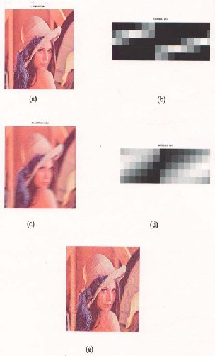
Fig 6: Blind Deconvolution Restoration results where a is the original image f(x, y), b is the original PSF h(x, y), c is the convolved image g(x, y), d is the guessed PSF h(x, y), e is the restored
image f(x, y) (MSE=393, PSMR=22).
[1] Gonzalez and Woods, “Digital Image
Processing” Fast Indian Reprint, 2002.
[2] Anil.K. Jain, “Fundamentals of Digital
Processing”. Prentice Hall of India-7 Reprint, 2001.
[3] V.K.Ananathashayana, “Image Representation using Number Theoretical Approach” PhD Thesis, University of Mysore,India.2001.
[4] A.K.Katsaggelos, Ed., Digital Image
Restoration. New York : Springer-Verlag, 1991.
[5] H.C.Andrews and B.R.Hunt, Digital Image
Restoration, Prentice-Hall, Inc., New Jersey, 1977.
[6] D.Kundur and D.Hatzinakos, “Blind image deconvolution revisited”, IEEE signal processing magazine, vol.13, no 3,, pp43-64, may 1996.
[7] How-lung and Kai-kuang Ma, “Noise Adaptive soft-Switching Median Filter”, IEEE Trans on Image Processing, vol.10,No 2, February 2001.
[8] Juan Liu and Pierre Moulin, “Complexity- Regularize Image Denoising”, IEEE Trans on Image Processing, Vol.10, No.6, June 2001.
[9] Georgios B.Giannakis and Robert W.Heath, “ Blind Identification of Multichannel FIR Blurs and Perfect Image Restoration, “IEEE Trans on Image Processing, Vol 9 No.11, November 2000.
[10] Deepa kundur, Dimtrios Hatzinakos, “Blind Image Restoration via Recursive Filtering using deterministic constrains”, IEEE Trans on Image Processing, Vol 46, No.2, February 1998.
IJSER © 2015 http://www.ijser.org
International Journal of Scientific & Engineering Research, Volume 6, Issue 4, April-2015 1278
ISSN 2229-5518
[11] Vrhel and Unser, “Multichannel Restoration with a limited a prior information”, IEEE Trans on Image Processing, Vol 8, No.4, April 1999.
[12] Wirawan and Duhamel, “Multichannel High
Resolution Blind image Restoration”,
[13] Alex Acha and Shmuel Peleg, “Restoration of Multiple Images with Motion Blur in different directions.”
[14] Bogdan Smolka and Marek Szczepenski, “ Random walk approach to the problem of impulse noise reduction”.
[15] Yirong Shen and Rui Zhang, “ Image Blind
Deconvolution”.
[16] Hung-Ta Pai, “Multichannel Blind Image
Restoration” Ph.D Qualifying proposal.
[17] Refeal Molina and Katsaggelos, “ Multi Channel Image Restoration using compound models” IEEE trans on image processing 2001.
IJSER © 2015 http://www.ijser.org