International Journal of Scientific & Engineering Research, Volume 6, Issue 1, January-2015 210
ISSN 2229-5518
Compact Low-Cost Digital Medical Ultrasound
Imaging System
Mawia Ahmed Hassan
Abstract— The objective of this work is to develop a compact low-cost digital medical ultrasound imaging system that has almost all of its processing steps done on the PC side. The new system was implemented using Analog Devices ultrasound analog front end chipset interfaced to a Virtex-5 FPGA with an 8-lane PCIe interface. The system was plugged into a Pentium 3.0 GHz Core 2 Quad PC with 8 GB memory. The system using serial LVDS interface protocol to, allow the output from an ADCs to come as a serial bit stream with drivers on both the ADC and the FPGA to recover the parallel data. This alleviates the need for designing the sampling and the signal recovery filters while maintaining an optimal performance at significantly lower power consumption. The procedures for the system are: first the derivation of the analytical signal in our design has to be on the digital side. The Hilbert transform can be used to derive the analytical signal from its real part. The 24-tap FIR Hilbert transformed is design with acceptable normalized RMSE with the analytical form of the signal. The FIR Hilbert filter zero tap coefficients are not computed and therefore an order L
filter uses only L/2 multiplications .Second, downsample id done for a Hilbert transformed single channel signal from 50 MSPS to a mere 5 MSPS without losing any information to reduce the size of the data, Third: The processing steps which done in the PC side include: the beamforming steps (dynamic receive focusing, aperture growth and apodization), envelope detection and compress the dynamic range. The new system has the potential to lower the cost and speed up the development, thus offering new opportunities for more cost-effective systems.
Index Terms— Medical Ultrasound, Digital Beamforming, LVDS interface protocol, FPGA, FIR Hilbert transformed
1 INTRODUCTION
—————————— ——————————
ith the growing availability of high-end integrated analog front-end circuits, distinction between different digital ultrasound imaging systems is determined almost exclusively by their software component. Efficient implementations of digital ultrasound systems rely on embedded digital signal processing on FPGA with data conversion from oversampled 1-bit delta-sigma ADC to minimize the number of lines going into the FPGA. However, using of serial LVDS interface protocol allows a serial output with drivers on FPGA to recover the parallel data. This alleviates the need for designing the sampling and the signal recovery filters while maintaining an optimal performance at significantly lower power consumption. Moreover, PC-based implementations for sophisticated medical imaging technologies have emerged where powerful multi-core computational ability replaces expensive embedded processing systems. This approach reduces the overall cost of
the system as well as the speed of system development.
The objective of this work is to develop a compact low-cost
————————————————
Mawia A.Hassan- Sudan Universit of Science & technology- Biomedical
Engineering Department. E-mail: mawiaahmed@sustech.edu.
Mawia A. Hassan received his B.Sc. degree from the Biomedical
Engineering department at Sudan University of Science & Technology
in 2002. He recived his M.Sc. & Ph.D. degrees from the Biomedical
Engineering department at Cairo University in 2007 and 2011
respectively. He is currently the head of Biomedical Engineering
Department at Sudan university of Science & Technology. His research interests include medical imaging processing, analysis in particular MRI and ultrasound imaging, and multidimensional signal processing for biomedical applications.
PC-based digital ultrasound imaging system that has almost all of its processing done on the PC side. We used data acquired from a resolution phantom. This data is collected in IBE Tech Giza, Egypt. The new system [1] was implemented using Analog Devices ultrasound analog front end chipset interfaced to a Virtex-5 FPGA with an 8-lane PCIe interface. The system was plugged into a Pentium 3.0 GHz Core 2 Quad PC with 8 GB memory. The system using serial LVDS interface protocol to, allow the output from a ADCs to come as a serial bit stream with drivers on both the ADC and the FPGA to recover the parallel data. This alleviates the need for designing the sampling and the signal recovery filters while maintaining an optimal performance at significantly lower power consumption.
The procedures for the system are: first the derivation of the analytical signal in our design has to be on the digital side. The Hilbert transform can be used to derive the analytical signal from its real part. We design 24-tap FIR Hilbert transformed with acceptable normalized RMSE with the analytical form of the signal. The FIR Hilbert filter zero tap coefficients are not computed and therefore an order L filter uses only L/2 multiplications .Second, we downsample a Hilbert transformed single channel signal from 50 MSPS to a mere 5 MSPS without losing any information to reduce the size of the data, Third: The processing steps which done in the PC side include: the beamforming steps (dynamic receive focusing, aperture growth and apodization), envelope detection and compress the dynamic range. A technique that expands the utility of current high-performance PCs to replace the high-cost embedded processing in digital ultrasound systems was studied.
IJSER © 2015 http://www.ijser.org
International Journal of Scientific & Engineering Research, Volume 6, Issue 1, January-2015 211
ISSN 2229-5518
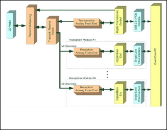
The main contribution of this work is to move almost all know-how related software components into the PC side of the system. The system block diagram for the system is shown in figure 1 where the data are collected and interfaced to the PC via a PCI-express bus through a Virtex-5 FPGA (Xilinx, Inc.). The use of several of these modules is possible through the use of multiple lanes of this interface bus.
Fig. 1. Block diagram of proposed digital ultrasound imaging system [1].
2 PREVIOUS METHODS
Several papers addressed the issues involved in digital beamformer design [2] [3] including the description of its main components. Embedded digital beamforming was initially done using Application-Specific Integrated Circuits (ASICs) [3]. Among the issues addressed is the sampling issue where a number of oversampled implementations were proposed to allow for artifact free conversion of ultrasound signals to the digital domain [3]. The phase aberration effect has also been described and its effects on ultrasound beamforming have also been assessed [3]. Many articles also addressed the digital signal processing algorithms that can be used in digital beamforming signal demodulation [2]. The issues involved in real-time digital ultrasound imaging are described in [4] including estimates for the computational complexity involved in each part of the ultrasound digital signal processing chain.
An interesting approach for efficient digital beamforming was presented in [5]. In their technique, a compact medical ultrasound beamformer architecture that uses oversampled 1- bit ADCs is presented. Sparse sample processing is used, as the echo signal for the image lines is reconstructed in 512 equidistant focal points along the line through its in-phase and quadrature components. That information is sufficient for presenting a B-mode image and creating a color flow map. The high sampling rate provides the necessary delay resolution for the focusing. The low channel data width (1-bit) makes it possible to construct compact beamformer logic. The signal reconstruction is done using FIR filters, applied on selected bit sequences of the delta-sigma modulator output stream. The approach allows for a multi-channel beamformer fitting in a single FPGA device. A 32-channel beamformer is estimated to
occupy 50% of the available logic resources in a commercially available midrange FPGA, and to be able to operate at 129
MHz. Simulation of the architecture at 140 MHz provides images with a dynamic range approaching 60 dB for an excitation frequency of 3 MHz. In spite of the interesting approach used, a number of significant issues can be raised in this method. First, the verification of the proposed methodology was done using computer simulations. The actual implementation of this method would involve dealing with such tricky issues as interfacing hardware to FPGA, printed circuit board design to minimize noise and cross talk between tracks of high-speed digital signals, as well as maintaining the power supply quality for the analog front-end with many fast switching digital signals in close proximity. Also, the justification of using oversampled 1-bit analog-to- digital converters in this work was to minimize the number of lines going into the FPGA. However, with the current analog- to-digital converter and FPGA technologies, another alternative has been the focus of most fast analog acquisition implementations in the past few years. This alternative is the use of serial LVDS interface protocol, which allows the output from an ADC to come as a serial bit stream with drivers on both the ADC and the FPGA to recover the parallel data. This alleviates the need for designing the sigma-delta sampling and the signal recovery filters for the oversampled 1-bit data stream while maintaining an optimal performance at significantly lower power consumption.
In this work, we take the following comments into account in planning for the new digital beamformer design. Moreover, we offer two additional advantages over this previous work, namely, the new integrated analog front-end components and the more powerful FPGA series that became available after this previous work was done.
3 METHODOLOGY
3.1 Data Compression Strategy
If we consider the process of collecting digital samples from a line with the maximum scanning depth of 22 cm, the number of samples collected by the 32 channel digital beamformer at the desired sampling rate of 50 MSPS at 12 bit resolution is about 894 kBytes. For a real-time acquisition of lines, the data rate entering the digital beamformer may reach up to 3.2 GBytes. It is not a trivial task to handle such huge amounts of data. Therefore, it is desired to somehow reduce such data without compromising the performance of the system.
The basic idea we developed to do that is based on the following points. First, the actual bandwidth of B-mode ultrasound imaging data in its quadrature form does not exceed a few MHz even with high frequency probes. Moreover, for Doppler ultrasound data, such bandwidth may even be as lower. The sampling done in hardware produces real samples and not the quadrature components representing the analytical form of each sample. It is difficult to have analog quadrature demodulation in the planned design because of the integration of the analog front end up until the ADC within one chip. Also, ultrasound signals before this chip are
IJSER © 2015 http://www.ijser.org
International Journal of Scientific & Engineering Research, Volume 6, Issue 1, January-2015 212
ISSN 2229-5518
too weak to process with this scheme. This of course in addition to the limitation of analog quadrature demodulation assuming narrowband nature for signals. This means that the derivation of the analytical signal in our design has to be on the digital side. Note that the Hilbert transform can be used to derive the analytical signal from its real part. With the analytical form of the signal, the signal can be downsampled to its bandwidth without aliasing while keeping the phase information intact for further phase-sensitive processing as wideband beamforming or Doppler shift estimation. Hence, for the ultrasound imaging situation, one can downsample a Hilbert transformed single channel signal from 50 MSPS to a mere 5 MSPS without losing any information.
3.2 Hilbert transform filter design
In the Hilbert transformation exact implementation, it acts like an ideal filter that removes all the negative frequencies and leaves all positive frequencies untouched. In its Matlab implementation, it is done using frequency domain filtering after the discrete Fourier transformation (DFT) is applied to the real signal. This ideal implementation affords high performance for broadband signals but at the same time requires high computational complexity (or FPGA resources in embedded implementations). Therefore, a number of authors suggested the use of digital finite impulse response (FIR) filter approximations to implement the Hilbert transformation. For linear time invariant (LTI) a finite impulse response (FIR) filter can be described in Equ. 1 [2]:
𝑀
𝑦[n] = 𝑏0 𝑥[𝑛] + 𝑏1 𝑥[𝑛 − 1] + ⋯ + 𝑏𝑀 𝑥[𝑛 − 𝑀] = � 𝑏𝑖 𝑥[𝑛 − 𝑖]. 1
𝑖 =0
Where x is the input signal, y is the output signal, and the
constants bi , i = 0,1,2,…,M, are the coefficients. The designed
FIR Hilbert filter can be used to generate the Hilbert
transformed data of the received echo signal. The impulse
response of the Hilbert filter with length N (odd number) is defined as in Equ. 2 [6]:
2 sin2 (𝜋(𝑛 − 𝛼)⁄2)
Given the frequency characteristics of most ultrasound probes having around 60% bandwidth around the center frequency, the frequency spectrum of the signal is sparse with a significant part of the spectrum having negligible signal components. So, it is possible to exploit this signal characteristic to make a dramatic reduction in signal bandwidth while maintaining the original information intact. Using a discrete FIR Hilbert transform filter, the analytic signal can be computed with only the positive side of the original signal spectrum. Hence, such analytic signal can be downsampled to only the bandwidth of the analytic signal, which is much smaller than that of the real signal.
Digital finite impulse responses (FIR) filter approximations to implement the Hilbert transformation. Even though simple filters can be used with accuracy/filter length trade-off, the computational complexity of working on the original high sampling rate is still not practical for direct implementation. For example, for a 24-tap FIR filter implementation of the Hilbert transformation, it is still a cumbersome task to implement several filters with an input and output data rate of
50 MSa/S. This complexity can be significantly reduced by combining the downsampling and filter implementation together. If we plan to downsample the analytical form of the data after the filter, it makes no sense to compute 50 MSPS in the output when we indeed plan to throw away 95% of them. Therefore, the Hilbert FIR filters are designed as multirate filters in such a way to do both the filtration and downsampling at the same time. For the above example, for an analytic signal bandwidth of 5 MHz, the filter outputs only
5 MSa/s per channel rather than 50 MSa/s.
The analytic signal consists of the original real signal
decimated by the factor of choice and the output of the
multirate Hilbert filter that output a decimated version of the
imaginary part of the signal. The Hilbert filter is implemented
in the common optimized form whereby the zero tap
coefficients are not computed and therefore an order L filter uses only L/2 multiplications. Also, the coefficients are implemented as 16-bit signed integers. Given that the same coefficients are used for all channels, it is possible to use a
ℎ[𝑛] = �𝜋


𝑛 − 𝛼 , 𝑛 ≠ 𝛼, 2
0 , 𝑛 = 𝛼
longer FIR Hilbert filter for multiple channels in an interleaved manner. In this case, the signal outputs for different channels sustain small delay differences that can be
α = (N − 1)/2. We chose the filter length equal 16,20,24,28 and
32 with a Hamming window used to reduce the sidelobe
effects. According to the normalized root mean square error
(RMSE) between the designed filter and ideal Hilbert
transform filter. The values of the RMSE for the five FIR filters
are equaled 0.0109, 0.0096, 0.0092, 0.0091, and 0.0090. The 24-
tap FIR filter is selected because it provided a medium RMSE.
3.3 Data processing strategy
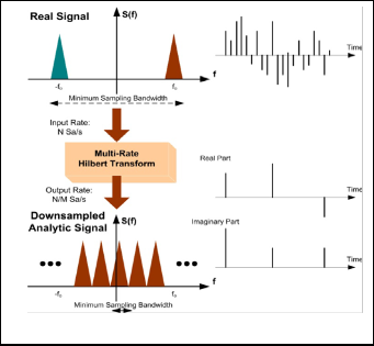
The goal of this section is to describe the method used to reduce the required raw ultrasound data transfer bandwidth while maintaining the phase information. The processing steps are shown in Figure 2 for single channel data (with other channels using the same architecture). Assuming that the sampling rate of each channel is N Sa/s, the acquired samples represent an oversampled version of the real part of the signal.
easily compensated in the further beamforming stage of the system.
3.4 The beamforming steps
3.4.1 Dynamic receive focusing for curve linear array
The dynamic focusing is the process of changing the receive focal distance of an array transducer assembly dynamically [2]. Figure 3 was shown the geometry which is used to determine the channel and depth-dependent delay of a focused curve linear array transducer. Because the probe used in the first data is curve linear array it must be correct the aperture coordinates.
Table 1 shows the probe General Specifications used in the first data. The angular step θ in radians is equal to the probe pitch over Radius of Curvature (ROC). Calculate the center of each element as a rotation of the center line from the geometry
IJSER © 2015 http://www.ijser.org
International Journal of Scientific & Engineering Research, Volume 6, Issue 1, January-2015 213
ISSN 2229-5518
using the rotation matrix Rθ (Equ. 3):
𝑐𝑐𝑐θ −𝑐𝑖𝑛θ
�𝑐𝑖𝑛θ 𝑐𝑐𝑐θ
This rotates column vectors by means of the
following matrix multiplication (Equ. 4):
′
TABLE 1
THE PROBE GENERAL SPECIFICATIONS


Array Geometry Type Curved Linear Array
Nominal Center Frequency 3.5 MHz
𝑥𝑛
𝑐𝑐𝑐θ −𝑐𝑖𝑛θ
𝑥𝑛
Pitch 0.516 mm
�𝑦′ � = �𝑐𝑖𝑛θ 𝑐𝑐𝑐θ � �𝑦𝑛 �, 4
Where n=1,2,3,…,number of elements in aperture. So the
Number of Elements 128 ea
Radius of Curvature 38.41 mm
′ ′ Elevation Aperture 12.5 mm
coordinate's correction (xn , yn) of the point (xn , yn) after
rotation are (Equ.6-5 and 6):
′
Elevation Focus 50 mm

Field of View 76.73 deg
𝑥𝑛 = 𝑥𝑛 cos θ − 𝑦𝑛 sinθ.
𝑦′ = 𝑥 sin θ + 𝑦 cosθ.
5
6 Then move the origin to the center of the probe (xi ,yi) by
subtract y' from the ROC. After the coordinates correction we
apply the dynamic focusing to the aperture. After a wave-
front is transmit into the medium an echo wave propagates
back from the focal points P1 (x1 ,y1), P2 (x2 ,y2),….. Pm
(xm,ym) to the transducer. The depth step used to calculate
the focal points coordinates equal to the depth over number
of points in image (Number of samples/Undersampling
factor. xn =0, yn =m× depth step. (m=0, 1,2,3,…, number of
points in image).
After we calculated the coordinates of the aperture and focal
points (P), the distance from Pm (xm,ym) to the aperture
′ ′
coordinates (xn , yn) is given by:

′ 2 ′ 2 7
𝑡 = 1/𝑐�(𝑥𝑛 − 𝑥𝑚 )
+ 𝑦𝑛 − 𝑦𝑚 ) .
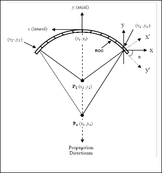
Fig. 2. Sampling Strategy [1].
Fig. 3. Geometry of a focused transducer array..
Then the delays converted to number of samples by divided the delays by the sampling time.
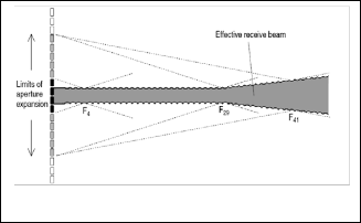
3.4.2 Aperture growth and apodization
The aperture means the size of the transducer surface used for producing the ultrasound beam and detecting echoes for each beam lines. We increase the number of receiving elements in the transducer array by increasing the number of aperture size with depth (figure 4), that keeping the lateral resolution nearly constant. The best lateral resolution if there is a large aperture and short wave length (high frequency) and also depend on the F-number which equals two.
Apodization is amplitude weighting of normal velocity across the aperture [7], one of the main reasons for apodization is to lower the side lobes on either side of the main beam [8]. Just as a time side lobes in a pulse can appear to be false echoes [7]. Aperture function needed to have rounded edges that taper toward zero at the ends of the aperture to create low side lobes levels. We used Hanning window as apodization function to reduce the side lobes.
For compensate for attenuation in the medium we apply the time gain compensation (TGC) curve in figure 5 with 255 is the maximum of the curve and 1 is the minimum of the curve.
3.4.3 Envelope detection and compress the dynamic range
The analytic envelope of the signal is calculated as the square root of the sum of the squares of the real and quadrature components [9,10,11]. The envelope can be
IJSER © 2015 http://www.ijser.org
International Journal of Scientific & Engineering Research, Volume 6, Issue 1, January-2015 214
ISSN 2229-5518
calculated from Eqi. 8 [12]:

𝐴(𝑡) = �𝐴𝐼 2 (𝑡) + 𝐴𝑄 2 (𝑡) .
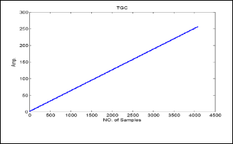
Fig. 4. Aperture growth..
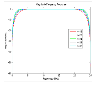
Fig.5. Aperture growth..
4 RESULTS
8
4.1 The ultrasound Data
The system was used to acquire data from a resolution phantom. The data acquired from a resolution phantom. This data is collected in IBE Tech Giza, Egypt.The sampling rate was 50 MHz and the number of channels used acquired was
32. The scan depth was 6 cm. the number of channels was 32 channels, and the ADC sampling rate was 50 MSPS. Curve linear array shape transducer was used to acquire the data with center frequency of 3.5 MHz, and element spacing of
0.516 mm. Each ultrasonic A-scan was saved in a record consisted of 4096 RF samples per line each represented in 2 bytes. The speed of the ultrasound in the phantom was 1540 m/sec.
4.2 Experimental verification
The PCIe interface bandwidth did not allow real-time raw data transfer to the PC for processing because of several efficiency problems that did not permit the system to reach its peak transfer rate (such as packet size). The transfer rate was significantly boosted by using the compression strategy
above. In Figure 6.2, the data from a single channel centered
above one of the pins in the scanned phantom is shown.
The frequency response of apply 16-, 20-, 24-, 28-, and 32-
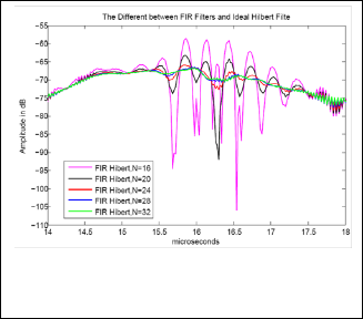
tap FIR Hilbert filter shown in Figure 6. Figure 7 had shown
the different between the FIR Hilbert filters and the ideal
Hilbert filter. The values of the RMSE for the five FIR filters
are equaled 0.0109, 0.0096, 0.0092, 0.0091, and 0.0090. From the
result 24-tap provided a good result because it gave the RMSE
look like random signal and had medium RMSE value between the five selected FIR filters.
Where AI , AQ is the magnitude of the in-phase and quadrature components and A(t) is the envelope (magnitude) of the received echo at time t.
The envelope then compressed logarithmically to achieve
the desired dynamic range for display (8 bits). It is typical to
use a log compressor to achieve the desired dynamic range for
display. Log transformation compressed the dynamic range
with a large variation in pixels values [13].
3.4.4 PC processing
Given that the number and geometry of ultrasound scan lines vary with probe and in all cases are different from what practical image display requires. It is necessary to perform a scan conversion step to reconstruct the ultrasound image. In its most general form, this step takes raw ultrasound lines along with their geometrical properties (i.e., direction, spacing, etc.) and estimates a rectilinear array of values representing the image that is compatible with the display device. The specifications of our design require the image to be a 512×512 matrix of values. This step is done in real-time on the PC used to display the image.
Fig.6. Magnitude frequency responses for FIR Hilbert filter with filter length equal to 16,20,24,28,and 32.
IJSER © 2015 http://www.ijser.org
International Journal of Scientific & Engineering Research, Volume 6, Issue 1, January-2015 215
ISSN 2229-5518
Notice that the downsampling was preceded by an antialiasing filter implemented as an FIR digital filter and combined with the Hilbert transform to reduce the noise superimposed from other frequencies in the downsampling step. This step has the drawback of increasing the complexity of the Hilbert.
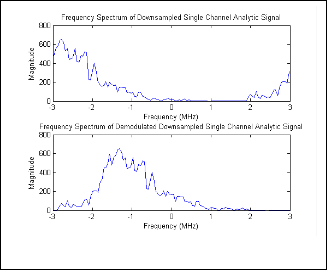
Fig.7. The different between the FIR Hilbert filters and the ideal Hilbert filter transform..
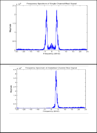
The results of applying the 24-tap FIR Hilbert transform to compute the analytic signal is shown in Figure 8 (b) where the frequency spectrum of the signal is computed and shows a single sided spectrum for the analytic signal compare to the frequency spectrum of the real signal in figure 8 (a). The spectrum after applying a divide-by-8 downsampling step is shown in Figure 9 before and after the required demodulation.
Fig .9. Frequency spectrum of downsampled analytic signal before and after the demodulation step.
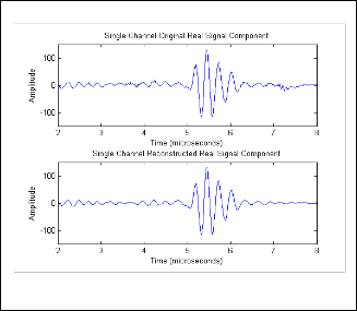
To show that this processing strategy did not cause information loss, the real signal was reconstructed and compared to the original as shown in Figure 10. The error between the two signals was lower than 1% for this particular experiment but increases to nearly 10% without the antialiasing filter.
(a)
Fig .10. Reconstructed and original real signals.
(b)
Fig .8. Frequency spectrum. (a) Frequency spectrum of
real signal,(b) Frequency spectrum of analytic signal.
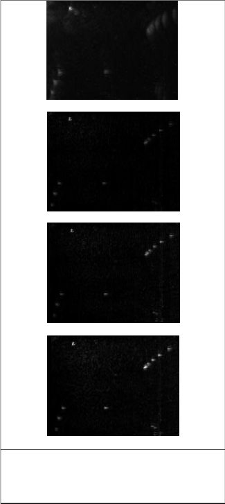
Once the data were in the PC memory, reconstruction of final image was done using spatially variant filtration of the received line data implemented using a look-up table. In Figure 11(a,b,c, d), a magnified 2cm × 1.5cm part of the image containing the resolution pins is shown without focusing, with (dynamic focusing, dynamic aperture, and apodization), after
IJSER © 2015 http://www.ijser.org
International Journal of Scientific & Engineering Research, Volume 6, Issue 1, January-2015 216
ISSN 2229-5518
apply TGC , after envelope detection and compress the dynamic range respectively.
(a) (b) (c)
(d)
Fig .11. Zoomed part of the reconstructed image. (a) Without focusing, (b) with dynamic focusing, dynamic aperture, and apodization, (c) After apply TGC, (d) After envelope detection and compress the dynamic range.
data The new system has the potential to lower the cost and speed up the development, thus offering new opportunities for more cost-effective systems.
REFERENCES
[1] A. M. Hendy ,M. A. Hassan, R. Eldeeb, D. Kholy, A. Youssef and Y.
M. Kadah, “PC-Based Modular Digital ultrasound Imaging system,” in
Proc. IEEE Ultrason. Symp., pp.1330-1333,Rome, Italy, September 2009. [2] B.D. Steinberg, “Digital beamforming in ultrasound,” IEEE Transactions on Ultrasonics, Ferroelectrics and Frequency Control, vol. 39, no. 6, pp.716-
721, 1992.
[3] C. Fritsch, M. Parrilla, T. Sanchez, O. Martinez, “Beamforming with a reduced sampling rate,” Ultrasonics, vol. 40, pp. 599–604, 2002.
[4] C. Basoglu, R. Managuli, G. York, and Y. Kim, “Computing requirements of modern medical diagnostic ultrasound machines,” Parallel Computing, vol. 24, pp. 1407-1431, 1998.
[5] B.G. Tomov and J.A. Jensen, “Compact FPGA-Based Beamformer Using
Oversampled 1-bit A/D Converters,” IEEE Transactions on Ultrasonics, Ferroelectrics and Frequency Control, vol. 52, no. 5, pp. 870-880, May
2005.
[6] S. Sukittanon, S. G. Dame, “FIR Filtering in PSoC™ with Application to Fast Hilbert Transform,” Cypress Semiconductor Corp., Cypress Perform, November 2005.
[7] Szabo, T. L., Diagnostic Ultrasound Imaging: Inside Out, Elsevier Academic
Press: Hartford, Connecticut, 2004.
[8] J. Synnevag, S. Holm and A. Austeng, “A low Complexity Delta- Dependent Beamformer,” in Proc. IEEE Ultrason. Symp., pp.1084-1087,
2008.
[9] J. O. Smith, Mathematics of the Discrete Fourier Transform (DFT), Center for
Computer Research in Music and Acoustics (CCRMA), Department of
Music, Stanford University, Stanford, California, 2002.
[10] P. Montuschi and M. Mezzalama, “Survey of square rooting algorithms,”
in Proceedings of the IEEE. 137, 31–40, 1990.
[11] J. Prado and R. Alcantara, “A fast square-rooting algorithm using a digital signal processor,” in Proceedings of the IEEE. 75, 262–264, 1987.
[12] T. K. Song and S. B. Park, “A new digital phased array system for dynamic focusing and steering with reduced sampling rate,” Ultrason. Imag. 121–16,
1990.
[13] R. C. Gonzalez, R. E. Woods, Digital Image Processing, Pearson Prentice
Hall, Upper Saddle River, New Jersey, 2008.
4 CONCLUSION
Compact low-cost digital medical ultrasound imaging system that has almost all of its processing steps done on the PC side is presented. Downsample id done for a Hilbert transformed single channel signal from 50 MSPS to a mere 5
MSPS without losing any information to reduce the size of the
IJSER © 2015 http://www.ijser.org