
International Journal of Scientific & Engineering Research Volume 4, Issue 2, February-2013 1
ISSN 2229-5518
Classification of Software Projects using k- Means, Discriminant Analysis and Artificial Neural Network
R. Chandrasekaran and R. Venkatesh Kumar
Abstract— An attempt is made in this paper to identify the groups of software development projects which demonstrate the significance of comparable characteristics based on various parameters associated with the Source Lines of Code (SLOC). Initially, software projects are clustered by using k-means cluster analysis. These groups are investigated further with the Discriminant Analysis (DA) and compared with Artificial Neural Network (ANN). For this purpose, we collected the historical data of software development projects from one of the major information technology (IT) company and this provided essential progressive information such as Planned Value (BCW S), Actual Cost (ACW P), Earned Value (BCW P), Cost Performance Index (CPI), Average Team Size (Team_Size) and Source Lines of Code (LOC).The results of this comparison study indicate that a Statistical model based on discriminant analysis is marginally better for prediction of the effort, than a non-parametric model based on artificial neural network. The classification method proposed in this paper may be used to identify the similar category of projects and for forecasting the software development cost and time effort. Hence, this approach would be useful for planning and preventive actions in the process of software development. The Statistical Software Package IBM SPSS 19.0 is used for the present analysis.
Index Terms — Artificial Neural Network, Cluster Analysis, Discriminant Analysis, k-Means, Lines of Code, software development estimate and Software Effort Estimation.
—————————— ——————————
It is of utmost important for both customers and the software companies to plan and predict certain parameters for any new project at the proposal stage to get beneficial results. Hence any Software Project Manager would be interested to determine the software development cost and effort, which will help them to allocate the budget, decide the time line, plan the resource and risks, so that an optimal operational metrics is obtained (Lionel, Victor, and Yong, 1994).Software Development Life Cycle (SDLC) is presented in Figure 1. It is essential to get the accurate cost and effort estimation for the project proposal to obtain mutual benefits. In order to evaluate cost and effort, we have to accumulate metrics from the previous projects and compare the similar characteristics with the current projects. For this purpose, many software effort estimation models have been proposed in the software
project managers to take the correct decision.

Estimation is a crucial activity for successful software project management, since this is very fundamental for budgeting and project planning. The quality of the estimation is one of the factors, which determines the success of the project and facilitate to avoid the risks. Inaccurate estimations have frequently to lead to the failure of the projects. In general, within budget and On-time deliverables are important concern for the software organizations. Under-estimated projects can have unfavourable outcome on business, performance and competitiveness. Over-estimated projects can result in poor resource allocation and missed business opportunities to take on new project.
industry. In general, Software Effort Estimation Models fall under following two categories: (1) Algorithmic models such as SLIM, COCOMO, Multiple Regression, Statistical models, etc… and (2) Non-Algorithmic models such as Fuzzy Logic (FL) Neural Network (NN), Case-Base Reasoning (CBR), Regression Trees, etc…, (Wittig and Finnic, 1994) in order to identify the optimal estimation model and helping software
Project Initiation
System Concept
Development
Integration and
Testing
Implementations
Design &
Development
Operations & Maintenance
————————————————
R. Chandrasekaran, Associate Professor and Head (Retd.), Department of
Statistics, Madras Christian College, Tambaram, INDIA – 600 059.
Project Planning Requirements
Analysis
Disposition
Fig 1. Software Development Life Cycle
The main objective of this research is to identify the similar groups of software development projects which share similar
IJSER © 2013 http://www.ijser.org
International Journal of Scientific & Engineering Research Volume 4, Issue 2, February-2013 2
ISSN 2229-5518
characteristics based on the Effort of Lines of Code (LOC) by performing k-means clustering method. The data set used in this research is based on the historical development projects data from one of the major information technology (IT) company. The clusters obtained through the k-means clustering method is further investigated and validated through the use of Discriminant Analysis (DA) and Artificial Neural Network (ANN). These methods are implemented using Statistical Software Package IBM SPSS 19.0.
This paper is structured as follows:
Section 2 Provides the literature review about the Software effort estimation, Cluster analysis, Discriminant Analysis and Artificial Neural Network.
Section 3 Includes a description about Cluster analysis
Section 4 Provides a brief explanation about Discriminant
Analysis.
Section 5 Includes a brief account of Artificial Neural
Network.
Section 6 Exhibits a method for classification of software development projects and Comparison of Discriminant Analysis and Artificial Neural Network study.
Section 7 Presents conclusion of the present research.
Shepperd et al. (1996), classification of estimation and prediction techniques can be categories into three ways, which are algorithmic models, expert judgment and machine learning. This work mainly focuses on combining clustering using machine learning techniques. The different types of clustering methods have already been applied to several aspects of software project management, including software effort/schedule estimation, software metrics and software quality.
Discriminant Analysis (DA) can be classified as three types, namely, direct, hierarchical and stepwise. Kinnear and Gray (2001) has highlighted that direct Discriminant Analysis involves all the variables entering in the equations at once, whereas, in hierarchical Discriminant Analysis, the variables enter in the equation according to a schedule set by the researcher, and in stepwise Discriminant Analysis statistical criteria are used in determining when the variables will enter the equations.
A cluster analysis is used to identify the small, medium and high risk of software projects. Risk measurements across the levels exposed that, even low risk projects have a high level of complexity risk (Linda et al., 2004). It is associated with requirements and planning. The results suggest that, Project scope have an effect on all dimensions of risk. There are past
studies about software project effort estimation on cost overrun (Procaccino, et al., 2002 and Verner, et al., 2007). The logistic regression is also used to predict the delay delivery of software projects (Takagi, et al., 2005).
The Software defect prediction models will change from environment to environment pertaining to specific defect patterns, but it does not mean building common defect prediction model (Koru and Liu, 2005). In fact, such models would be really useful and provide a starting point for development environments with no historical data. Stockburger (2007), specified the use of discriminant function to forecast group membership of a project.
Cluster analysis is an unsupervised classification method. Generally, it is useful in many research areas such as Statistics, data mining, data classification, pattern recognition and machine learning. The main objective of the cluster analysis is to partition large dataset into smaller groups such that objects within a group are similar while objects between the groups are dissimilar, in some sense. Even though there are different methods available to solve the clustering problem, the most commonly used method is k-means clustering, which is a simple and efficient partition method developed by Mac Queen in 1967 (Zhang, et al. (2006); Li and Wu, 2007 and Ye, et al., 2008).
Software Testing is the most important part in the Software Development Life Cycle. Software projects testing activities used at least 30 percent of the project overall effort. Software project testing is an essential part to ensure the software product quality (Sonali and Shaily, 2010). There is always a rigid Schedule during the software system development, thereafter reducing efforts of performing software testing management. Ogunsanmi, et al., (2011), conducted a study for various risk sources in Design and demonstrated that the projects can be classified into three risk groups of cost, time and quality using the discriminant analysis technique.
Cluster analysis is a statistical technique for identifying groups of objects using measurements on them (Li and Wu,
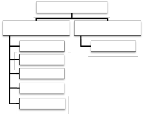
2007). The main purpose of a cluster analysis is to classify a sample of objects based on the measured variables into a number of different groups such that similar objects are placed in the same group (Manly, 2005). The clustering algorithms are generally classified into two types, which are hierarchical and non-hierarchical algorithms (Anderson, 2003), as depicted briefly in Fig 2.
IJSER © 2013 http://www.ijser.org
International Journal of Scientific & Engineering Research Volume 4, Issue 2, February-2013 3
ISSN 2229-5518
Cluster Algorithms
function (Jain and Dubes, 1998).The squared sum error (SSE)
of a partition K = (k1, k2, …, km) is defined as:
Hierarchical methods
Non-Hierarchical methods
m nj 2 j
SSE (K) = ∑j=1 ∑i=1 d (Qi, fj )
(1)
Single Linkage
K- Means
nj j
nj j
∑k=l Qkl
∑k=l Qkm
Complete Linkage
![]()
f =
nj
, … ,
![]()
nj
j j j
Average Linkage
Ward’s Method
Centroid method
Fig 2. Cluster Algorithms
Hierarchical clustering is one of the most popular methods and it can be either agglomerative or divisive (Anil and Richard, 1998). Agglomerative hierarchical clustering is called as bottom-up clustering method. It starts with each case being a cluster into itself and similar clusters are merged. The algorithm ends with all objects in a same cluster. Divisive Hierarchical Clustering is called as top-down clustering method. It works in the opposite direction of agglomerative clustering method. It starts with a single cluster holding all the objects, then sequentially splitting objects until every object is in a separate cluster.
In general, Non-hierarchical cluster analysis is used when huge quantity of data is involved (Anil and Richard, 1998). It is a most common method because it allows subjects to move from one cluster to another cluster and these features are not possible in the hierarchical cluster method. The number of clusters (k) should be specified in advance in the k-means clustering technique.
Initially, select k objects randomly from the dataset, which correspond to k-cluster centers.
Assign each object to the cluster with which it has minimum distance.
Calculate the mean value of the objects for each cluster, to update the centroids.
Repeat these steps until no changes in the centroid/ no relocation of objects occur.
Once achieved a “high-quality” partition of objects corresponding to optimizing a measure function defined either locally or globally, the algorithm stops (Rencher, 2002). The k-means algorithm tries to minimize the squared error
where the cluster kj is a set of objects (Q1 , Q2 , … , Qn ) and fj is
the centroid of kj. Therefore, the k-means algorithm minimizes
the distance between the intra-cluster (Anil et al., 1998).
The main disadvantages of K-means cluster are:
The performance of the algorithm depends on the initial centroids. So, there is no assurance for an optimal solution.
The user has to identify the number of clusters in advance.
Discriminant Analysis (DA) is used for predicting group membership based on a linear combination of independent variables. The method of combining independent variables into a single new variable is called as discriminant function (Ogunsanmi, et al., 2011). The concepts of discriminant function is well documented by Stockburger (2007), and Kinnear and Gray (2001).
The efficiency of discriminant function is tested with a Statistic, known as Wilks Lambda (^). This measure indicates the significant difference between the target groups (Kinnear and Gray, 2001). The Discriminant function is expressed as follows.
D = w1X1 + w2X2 + w3X3 + … +wiXi + a (2) Where D = Discriminate function;
wi = Weight for the i-th variable
Xi = Score for the i-th variable; a = Constant
Discriminant function is similar to the regression equation. The wi’s are unstandardized discriminant coefficients. This wi’s maximize the distance between the means of the dependent variable. Good predictors tend to have large weights.
Artificial Neural Networks are relatively crude electronic models similar to the neural structure of the brain. In other words, Artificial Neural Network (ANN) is immensely parallel adaptive network of simple nonlinear computing elements called Neurons (Fig: 3). An artificial neural network comprises of eight basic components : (i) neurons, (ii) activation function, (iii) signal function, (iv) pattern of connectivity, (v) activity aggregation rule, (vi) activation rule,
IJSER © 2013 http://www.ijser.org
International Journal of Scientific & Engineering Research Volume 4, Issue 2, February-2013 4
ISSN 2229-5518
(vii) learning rule and (viii) environment (Jagannath and
Bibhudatta, 2011).
(Jagannath and Bibhudatta, 2011): Steps in effort estimation:
1. Data Collection: Collect development project data from
X1 Wk
Activation
previous projects like Planned Value (BCWS), Actual Cost (ACWP), Earned Value (BCWP), Cost Performance Index (CPI), Average Team Size (Team_Size) and Source Lines of
X2 Wk
Xm Wk
Aggregation Rule
Output
Code (LOC)
2. Division of dataset: Divide the number of data into two parts – Training (75%) &Testing (25%).
3. Design: Design the neural network (NN) with number of neurons in input layers same as the number of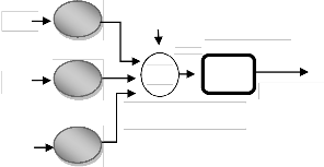
Fig 3. Architecture of Artificial Neural Network
In mathematical notation, any neuron-k can be represented as follows;
characteristics/attributes of the project.
4. Training: Feed the training data set to train the neural network.
uk = ∑m 1 wkj xj
(3)
5. Validation: After training is over then validate the NN
yk= <p (uk + bk ) (4)
where X1, X2, …, Xm are the inputs, Wk1, Wk2, … , Wkm are the
synaptic weights of the corresponding neuron, uk is the linear
combiner output, bk is bias, φ() is the activation function and
yk is the output (Jagannath and Bibhudatta, 2011).
Artificial Neural Network is used to obtain effort estimation due to its ability to learn from historical data (JaswinderKaur and Karanjeet, 2010). This also helps to model complex relationships between the dependent (SLOC) and independent variables (Effort Drivers). It has the ability to simplify from the training data set thus enabling it to produce acceptable result for previously unseen data.![]()
Input Layer Hidden Layer Output Layer
![]()
![]()
BCWS
Interce
with the validation data set.
6. Testing: Finally test the created NN by feeding test dataset.
7. Error calculation: Check the performance of the ANN. If acceptable then stop, else again go to step (3), make some changes to the network parameters and proceed.
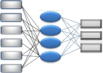
The RBF procedure fits a radial basis function neural network, which is a feed forward, supervised learning network with an input layer, a hidden layer called the radial basis function layer, and an output layer (Figure 4). The hidden layer transforms the input vectors into radial basis functions. The RBF procedure performs prediction and classification similar to the MLP procedure. To classify the software projects, the paper focuses on Radial Basis Function (Jagannath and Bibhudatta, 2011).
ACWP
BCWP CPI Team_Size
SLOC
pt
H(1) H(2)
H(3)
LARGE MEDIUM
SMALL
The RBF procedure trains the network in two stages:
The procedure determines the radial basis functions using clustering methods. The center and width of each radial basis function are determined.
Given the radial basis functions, the procedure estimates the synaptic weights. Sum-of-squares error function with identity activation function for the output layer is used for both prediction and classification. Ordinary Least Squares regression is used to minimize the sum-of-squares error.
Fig: 4. Radial Basis Function ANN
Many different models of neural nets have been proposed for solving numerous complex real life problems. The 7 steps for effort estimation using ANN can be summarized as follows
Due to this two-stage training approach, the RBF network is, in general, trained much faster than MLP.
IJSER © 2013 http://www.ijser.org
International Journal of Scientific & Engineering Research Volume 4, Issue 2, February-2013 5
ISSN 2229-5518
The main object of this research is to identify the similar group of effort spent for software development. We performed k-means cluster analysis, which is used to identify the underlying groups of software projects. Further, these groups are subjected to discriminant analysis and Neural Network. For this purpose, we obtained 810 historical software development project data, of which 75% has been used for training and 25% for testing purposes. Various parameters which are considered in this research are Planned Value, Actual
Cost, Earned Value, Cost Performance Index (CPI), Average Team
Size and Source Lines of Code (SLOC). The raw data set is
normalised before subjecting it to analysis. The best possible 3 groups of projects (called Small, Medium and Large) has been identified using k-means algorithm and the results are presented in Table1 with the Final Cluster Centers. These two methods are implemented using Statistical Software Package
IBM SPSS 19.0.
Table 1. Final Cluster Centers
Variables | Cluster | ||
Variables | 1 | 2 | 3 |
Planned Value Actual Cost Earned Value Cost Performance Index Average Team Size Source Lines of Code | 0.03 0.06 0.04 0.18 0.18 0.02 | 0.01 0.02 0.02 0.18 0.03 0.01 | 0.01 0.02 0.01 0.26 0.03 0.01 |
These 3 groups (1-LARGE, 2-MEDIUM, 3-SMALL) obtained were further investigated with discriminant analysis (DA) and Neural Network (NN). It could assist the decision makers to identify similar types of development projects, with best effort estimation, to develop the code and test the project.
Table 2. Summary of Canonical Discriminant Functions
that would result from a one-way ANOVA on the first discriminant function. According to the result 67% of the variability of the scores for the first discriminant function is accounted by differences among the 3 groups which are Large, Medium and Small level projects. Similarly, Functions 2 has canonical correlation r = 0.70, therefore, 49% (0.70 = 0.49) of the variability of the scores for the second discriminant function is accounted for by the effort factors.
Table 3. Wilks' Lambda
Test of Function(s) | Wilks' Lambda | Chi- square | df | Sig. (p-value) |
1 through 2 2 | 0.166 0.504 | 1078.907 411.961 | 12 5 | 0.000 0.000 |
The output for significance tests and strength of relationship statistics for the discriminant analysis is shown in Table 3.The Eigen value of function 1 through 2 and function 2 have the p- values very close to zero (p= 0.000), indicating that the functions discriminate the groups.
The output for classification of groups is shown in Table 4. The classification results allow us to determine how well we can predict group membership using a classification functions.
The results indicate that:
Table 4. Classification of projects using Discriminant Function
Function | Eigen value | % of Variance | Cumulative % | Canonical Correlation |
1 2 | 2.031a 0.984a | 67.4 32.6 | 67.4 100.0 | 0.819 0.704 |
a. First 2 canonical discriminant functions were used in the analysis.
The results are shown in Table 2. Canonical Discriminant Function 1 has Eigen value2.031 and Function 2 has Eigen values 0.984. This implies that the function 1 has more variance between the groups and function 2 has lesser variance between the groups. The third column of this table indicates that the discriminant function 1 explains 67.4% of the variance between the groups while discriminant function 2 accounts for 32.6% of the variance. The last column of this table shows that the Function 1 has canonical correlation r =
0.82; by squaring the canonical correlation for this discriminant function (0.82 = 0.67), we obtain the eta square
a. 96.5% of selected Training grouped cases correctly classified.
b. 93.6% of unselected Testing grouped cases correctly classified.
For the training data, about 96.5% of the original group cases are correctly classified by this discriminant function.
For the testing data, around 93.6% of the original group cases are correctly classified by this discriminant function.
The output for group classification is shown in Table 5. The
IJSER © 2013 http://www.ijser.org
International Journal of Scientific & Engineering Research Volume 4, Issue 2, February-2013 6
ISSN 2229-5518
classification results allow us to determine how well we can predict group membership using a classification functions. Based on this study,
Table 5. Classification of projects using ANN
500
396 399
53 36
137
112
High Accepted Medium
Accepted
Small Accepted
Discriminant Analysis Neural Network
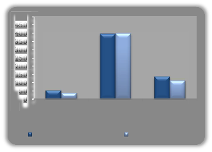
Fig 6. Training grouped cases correctly classified
Dependent Variable: Cluster Number of Case
For the training data set, about 90.10% of the original group cases are correctly classified by this ANN.
For the testing data, around 86.70% of the original group cases are correctly classified by this ANN.
There are few interesting and important facts about classification of Discriminant Function and Artificial Neural Networks (RBF).
It illustrates the predictive capability of each model. In the below table, out of 810 software development projects, 607
It illustrates the predictive capability of each model. In the below table, out of 810 software development projects, 203 (25%) projects used for testing purpose.
Table 7. Testing grouped cases correctly classified
Models | High Accepted | Medium Accepted | Small Accepted | Correct Classified Rate |
Discriminant Analysis | 15 | 136 | 39 | 93.60% |
Neural Network | 7 | 139 | 30 | 86.70% |
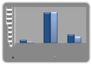
Testing data classified for the Discriminant Function at 93.60% and Artificial Neural Networks (RBF) at 86.70%, which implies that discriminant analysis gives better results than neural network analysis.
(75%) projects used for training purpose.
Table 6. Training grouped cases correctly classified
160
136 139
15 7
39 30
Training data classified for the Discriminant Function at
High Accepted Medium
Accepted
Small Accepted
96.50% and Artificial Neural Networks (RBF) at 90.10%, which implies that discriminant analysis shows better results than neural network analysis.
Discriminant Analysis Neural Network
Fig 7. Testing grouped cases correctly classified
In the Comparison study a statistical method of Discriminant Analysis is slightly better results than the non statistical method Neural Network.
IJSER © 2013 http://www.ijser.org
International Journal of Scientific & Engineering Research Volume 4, Issue 2, February-2013 7
ISSN 2229-5518
Estimation of Lines of Code (LOC) and required team size are essential parameters in the tasks of software project management. In the software development life cycle, project planning, effort/cost estimate, team size are made based on the code size. In this paper, we performed k-means clustering on software development projects and identified 3 groups, namely, Large, Medium and Small projects, of software development projects based on the Effort of Lines of Code (LOC). The clusters obtained are investigated with the discriminant analysis and Artificial Neural Network. The results of this comparison study indicate that a Statistical model based on discriminant analysis is marginally better for prediction of the effort, than a non-parametric model based on artificial neural network.
[1] Anil, K. J., and Richard C. D., (1998). Algorithms for clustering data, Prentice- Hall, Inc., New Jersey, USA.
[2] Anderson, T.W., (2003). An Introduction to Multivariate Statistical
Analysis, 3rd Edition, John Wiley, New York, USA.
[3] Jain, A., and Dubes, R., (1998). Algorithms for Clustering Data, Prentice
Hall, New Jersey, USA.
[4] JaswinderKaur, S., and Karanjeet, S., (2010). Neural Network-A Novel Technique for Software Effort Estimationl, International Journal of Computer Theory and Engineering, Vol. 2, No. 1,pp. 17-19.
[5] Jagannath, S., and Bibhudatta, S., (2011). Software Effort Estimation with Different Artificial Neural Network, International Journal of Computer Applications, Special Issue on “2nd National Conference, pp.
13-17.
[6] Kinnear, P. R., and Gray, C. D., (2001). SPSS For Windows Made Simple, Release 10, East Sussex, UK Psychology Press, Taylor and Francis Group
[7] Koru, A.G. and Liu, H.,(2005).Building Defect Prediction Models in
Practice, IEEE Software, Vol.22, No.6, pp.23-29.
[8] Li, C. and Wu, T., (2007). A clustering algorithm for distributed time series data, WSEAS Transactions on Systems, Vol.6, No.4, pp. 693-699.
[9] Lionel, C. B., Victor, R. B. and Yong-Mi. K., (1994). Change Analysis Process to Characterize Software Maintenance Projects, Proc. of the International Conference on Software Maintenance, Victoria, British Columbia, Canada, Vol.19, No.23, pp. 38-49.
[10] Linda, W., Mark, K., and Arun, R., (2004). Understanding software project risk: a cluster analysis, Information and Management , Vol.42, No.1, pp.115–125.
[11] MacQueen. J., (1967). Some methods for classification and analysis of multivariate observations, Proc. of the 5th Berkeley Symposium on Mathematical Statistics and Probability, pp. 281-297.
[12] Manly, B.F.J., (2005).Multivariate Statistical Methods: A primer, Third edition, Chapman and Hall.
[13] Ogunsanmi, O. E., Salako, O. A., and Ajayi, O. M., (2011). Risk Classification Model for Design and Build Projects, Journal of Engineering, Project, and Production Management, Vol.1, No.1, pp.46-
60.
[14] Procaccino. J., Verner, J., Overmyer, S., and Darter, M., (2002). Case study: factors for early prediction of software development success, Information and Software Technology, Vol.44, No.1, pp.53-62.
[15] Rencher, A.C., (2002), Methods of Multivariate Analysis, Second edition, Wiley, NY.
[16] Shepperd M., Schofield, C., and Kitchenham B., (1996). Effort estimation using analogy, Proc. of the 8th International Conference on Software Engineering, IEEE Computer Society Press, Berlin, pp.170-
178.
[17] Sonali, M., and Shaily, M., (2010). Advancements in the V-Model,
International Journal of Computer Applications, Vol.1, No.12, pp.29 –
34.
[18] Simon Haykin, (1998), Neural Networks: A Comprehensive Foundation, Second Edition, Prentice Hall.
[19] Takagi, Y., Mizuno, O., and Kikuno, T., (2005). An Empirical Approach to Characterizing Risky Software Projects Based on Logistic Regression Analysis, Empirical Software Engineering, Vol.10, No.4, pp.495-515.
[20] Verner, J., Evanco, W., and Cerpa, N., (2007). State of the practice: An exploratory analysis of schedule estimation and software project success prediction, Information and Software Technology, Vol.49, No.2, pp.181-193.
[21] Wittig, G.E. and Finnic, G.R., (1994). Using Artificial Neural Networks and Function Points to estimate 4GL software development effort, Australasian Journal of Information Systems (AJIS), pp. 87-94.
[22] Ye, Z., Mohamadian, H., Pang, S. and Iyengar, S., (2008). Contrast enhancement and clustering segmentation of gray level images with quantitative information evaluation, WSEAS Transactions on Information Science and Applications, Vol.5, No.2, pp.181-188.
[23] Zhang, Y., Xiong, Z., Mao, J. and Ou, L., (2006). The study of parallel k-means algorithm, Proc. of the 6th World Congress on Intelligent Control and Automation, pp. 5868-5871.
[24] Lu Luo, (2002). Software Testing Techniques, Technical Report, 17939A, Institute for Software Research International, Carnegie Mellon University, Pittsburgh, USA. http://www.cs.cmu.edu/~luluo/Courses/17939Report.pdf.
[25] Stockburger, D.W., (2007), Multivariate Statistics: Concepts, Models and
Application. Available at www.Mlto3m.
IJSER © 2013 http://www.ijser.org