International Journal of Scientific & Engineering Research, Volume 5, Issue 5, May-2014 1057
ISSN 2229-5518
An Insight into the Action Potential Generation in the Hodgkin-Huxley model
Dibya Thapa
Abstract— The brain is one of the most complex organ in the living being and for years its complexity has overwhelmed researchers, physiolo- gists and neuroscientists. Trying to map its behavior right from the start of evolution has brought about only little success. Here we have concen- trated on the basic unit of brain “neurons”. W hen the membrane potential reaches a certain threshold value spikes are generated. In this study we have applied concepts of computational modeling to the Hodgkin Huxley model equations which led to some interesting facts.
Index Terms— brain, Hodgkin Huxley, membrane potential, neurons , neuroscientists, spikes, threshold value .
—————————— ——————————
The Hodgkin Huxley (HH) model was developed by Alan
Hodgkin and Andrew Huxley in 1950’s for which they won
the 1963 Nobel Prize in the field of Physiology or Medicine.
Their experiments led to a series of five articles being pub-
lished in 1952 revealing the properties of ionic conductances
dominating the action potential. The final paper laid down the
framework for all the modern work in neural excitability [1],
[2].
Hodgkin and Huxley choose the squid axon which was
large enough to see and stick wires into. They threaded silver
wire inside the axon and by doing so they could measure the
electrical potential and deliver enough current to maintain a
particular voltage despite the efforts of ion channels in the
membrane to change it and this was known as voltage clamp
.This process gave them the idea about which current is being
passed through the membrane and in which direction. They
performed the same experiment in potassium or sodium free
solutions and by doing so under different voltage conditions
they could figure out how sodium and potassium currents
changed with the change in membrane potential. They then
used these collected data to construct the parallel conductance
wherein the electrical properties of segment of a nerve mem-
brane are modeled.
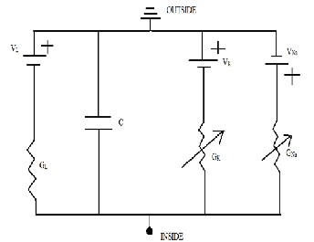
As we can see in fig 1 it consists of four parallel conducting
pathways connecting the inside and outside of the membrane.
Membrane capacitor and fixed membrane conductance are on
the left side. Resistor is connected to a battery and the batteries
are denoted by two parallel lines of different length, the long
line indicating the positive pole. The passive conductance in
this model is called as leak conductance and are not sensitive
to voltage hence the leak conductance remains same for all
voltage providing constant “leakiness” for current. Potential of
the battery with gleak is Eleak which is the major determinant of
resting potential and its short line is connected to the inside of
the membrane making the membrane inside negative [3],[4,[5].
————————————————
The right side consists of two active branches. The sodium battery and conductance and they are pointed in opposite di- rections. The potassium battery makes the membrane negative while the sodium battery makes it positive. The arrow in the conductance symbol under each battery means it is a rheostat. Sodium and potassium conductances are turned off at rest so that they don’t conduct which means at this time they have no effect on membrane voltage . If anyone is turned on, then as- sociated battery will dominate the membrane potential but if both are turned on at the same time the batteries will dis- charge massively overheat and blow up [1],[3],[6].
Fig 1: Parallel Conductance Model
IJSER © 2014 http://www.ijser.org
International Journal of Scientific & Engineering Research, Volume 5, Issue 5, May-2014 1058
ISSN 2229-5518
In the parallel conductance model current flowing is carried by the capacitor or by ions. As we can see the resistances re- lates to charge being carried by sodium and potassium ions and a leakage current. Using Ohm’s law (V=IR) the following equations were derived [7],[8].
IN a = gNa (V-VNa ) (1)
Again we have
gk =𝑔
k𝑛4 (10)
IK = gK (V-VK ) (2)
Il = gl (V-Vl ) (3)
Where gNa and gK depend on time and membrane potential. The values of VNa , VK , Vl, Cm and gL were determined via experimentation and are constants.
where 𝑔� 𝑘� is a constant, n is a dimensionless variable that var- ies from 0 to 1 and is the proportion of ion channels that are
open. In order to understand where n comes from we have the equation
To build their mathematical model they used the basic circuit equation![]()
dn = α
dt
(1-n)-βn n αn
, βn
are rate constants (11)
where
I = Cm
dv
![]()
+ I i
dt
(4)
where alpha ( α )is the rate of closing of the channels and beta (β) is the rate of opening. Hence together they give us the total rate of change in the channels during an action potential. Similarly the sodium conductance is described by the equation
I = the total membrane current density . I i = the ionic current density .
V=displacement of the membrane potential from its resting value.
gNa = m
𝑔RNa h (12)
Cm = the membrane capacity per unit area (assumed constant). t=time.
Further the ionic current was divided into a sodium current a potassium current and a leakage current primarily carried by chloride ions:
Ii = INa + IK +Il (5)
Here I Na means sodium current, I K means potassium current and I l meansleakage current. The model was further expanded by adding (1),(2),(3).
IN a = gNa (V-VNa ) (6) IK = gK (V-VK ) (7) Il = gl (V-Vl ) (8) V=V-VR (9)
VR denotes the resting potential.
where 𝑔RNa is a constant, m is the proportion of activating
sodium ion channels and h is the proportion of inactivation
of sodium ion channels. M and h can be further calculated
as
dm⁄dt= αm (1-m)-βm m (13)
𝑑ℎ⁄𝑑𝑑 =αh (1-h)-βh h (14)
alpha and beta (rate constants) can be calculated as:
n0 =𝛼𝑛𝑜 ⁄(𝛼𝑛𝑜 + 𝛽𝑛𝑜 ) (15)
(15)
αn = 0.01 (V + 10)/((exp (V+10)/10)-1) (16)
βN = 0.125 exp (V/80) (17) αm = 0.1(V+25)/((exp(V+25)/10)-1) (18) βm = 4exp(V/18) (19)
αh = 0.07exp(V/20) (20)
IJSER © 2014 http://www.ijser.org
International Journal of Scientific & Engineering Research, Volume 5, Issue 5, May-2014 1059
ISSN 2229-5518
βh = 1/(exp (V+30/10)+1) (21)
Therefore the final equation that we have is :
I= Cm 𝑑𝑑⁄𝑑𝑑 R + 𝑔Rk n V-VK ) + m 𝑔RNa h ( V-VNa ) + gl (V-Vl )
TABLE 1 PARAMETERS USED
(22)
4( 3
In order to mimic the behaviour of membrane potential we resort to simulation technique. Matlab was used for this pur- pose. As we can see “Fig 2” represents the evolution on mem- brane potential and spike generation in HH model. We dis- critize the time interval [0,T] into equal parts of size dt=0.01sec. Euler Maruyama method is applied to simulate the neuronal model. When the membrane potential reaches threshold voltage Vth in this case -70 a spike is generated and instantaneously the membrane potential is reset to its resting potential. Thereafter the membrane potential again evolves and reaches the threshold potential to generate another spike [9].Time interval between two consecutive spikes gives the Inter Spike Interval (ISI).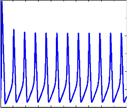
40
20
0
3.2 Addition of Noise
Noise and statistical fluctuations are present in all biological systems is now a well established fact. The main challenge across computational biology is understanding its role in cel- lular dynamics [4].So far we have come to know it can influ- ence information processing [5], spike time reliability [10], stochastic resonance [9], firing irregularity [11],[12], sub threshold dynamics [7],[9], and action potential initiation. During the past few years accurate methods for incorporating noise in the classical Hodgkin Huxley model have been devel- oped [13],[14],[15]. To introduce noise within a differential equation such as that of the HH model, we look for ways of introducing fluctuations into this deterministic system. The three main approaches are as follows [15],[16].
• Current noise
Replace (22) with
-20
I= Cm 𝑑𝑑⁄𝑑𝑑 + 𝑔Rk n
V-VK ) + m 𝑔RNa h ( V-VNa ) +
-40
-60
4 (
• Subunit noise
3
gl (V-Vl )+ ξv (t) (29)
-80
0 10 20 30 40 50 60 70 80 90 100
time
Fig2: Spikes generation with Vth= - 70
Replace (11), (13), (14) with
𝑑𝑑⁄𝑑𝑑 = 𝛼 Ry(1-y) – βy y + ξy(t) (30)
where y=n,m,h .
IJSER © 2014 http://www.ijser.org
International Journal of Scientific & Engineering Research, Volume 5, Issue 5, May-2014 1060
ISSN 2229-5518
40
20
0
-20
-40
0.14
0.12
0.1
0.08
0.06
0.04
0.02
-60
-80
0 20 40 60 80 100 120 140 160 180 200
time
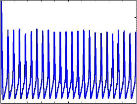
Fig 3: Change in the membrane potential with respect to time
0
4.3 4.35 4.4 4.45 4.5 4.55 4.6
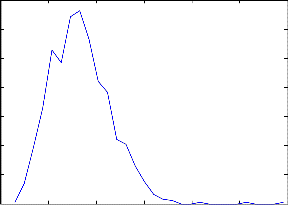
Fig 4: Probabilty Distribution Function of simulated ISI distribution
• Conductance noise
Replace (22) with
4
Hodgkin and Huxley not only helped scientists understand the concept of generation of action potential, they also laid down the framework for all the modern discoveries made in the field of computational neuroscience. In our quest of under- standing of the brain, it will be useful to concentrate on mod- els that suggest new and promising lines of experimentation,
3 at all levels of organization and the best model to choose
I= Cm 𝑑𝑑⁄𝑑𝑑 R + 𝑔Rk (n
+ ξ K (t)) (V-VK ) + 𝑔
RNa
(m h+ ξ
Na(t))
. ( V-VNa ) + gl (V-Vl ) (31)
“Fig 3” depicts the results of solving the HH model after the introduction of noise in the model equation.
3.3 Inter Spike Interval
The increase in the membrane potential of the neuron is due to the electrochemical processes inside the neuron [4], [10],[17]. FPT (first passage time) is the time epoch when the membrane potential reaches a certain threshold value for the first time. At this time a spike is generated and then the membrane poten- tial decays to a value known as resting potential. The first pas- sage time is generally random in nature [18]. Inter Spike Inter- val is the difference between time epochs of two consecutive spikes also known as ISI. Collection of ISI gives the probability distribution.
would be the HH model. We tried to understand how brains
compute, using computers to simulate and used our
knowledge from various fields such as mathematics, physics
and other computational fields.
References
[1] A.L. Hodgkin and A. F. Huxley, “A quantative description of. membrane current and its application to conduction and excitation in nerve”, J.Physiol, 1952.
[2] Jamie I. Vandenberg and Stephen G.Waxman, “Hodgkin and Hux- ley and the basis for electrical signalling: a remarkable legacy still going”, J Physiol 590.11 pp 2569–2570,2012 .
[3] P. Dayan and L.F Abbott: Theoretical Neuroscience “Computational and Mathematical Modeling of neural system”. MIT Press, 2001.
[4] Gerstner W, Kistler W M: Spiking Neuron Models: Single
Neurons,Populations, Plasticity: Cambridge University Press, 2001.
IJSER © 2014 http://www.ijser.org
International Journal of Scientific & Engineering Research, Volume 5, Issue 5, May-2014 1061
ISSN 2229-5518
[5] Shadlen M.N and Newsome W.T: “Noise, Neural Codes and
Cortical Organization, Current Opinion in Neurobiology”, vol-4,
1994, pp.569-579.
[6] Erik Skaugen and Lars Walloe, “Firing behaviour in a stochastic nerve membrane modelbased upon the Hodgkin-Huxley equations”, Acta Physiol Scand, 107: 343-363,1979
[7] Tuckwell, H. C. Introduction to theoretical neurobiology.
Cambridge, UK: Cambridge University Press; 1988.
[8] L. F. Abbott, “Lapicque’s introduction of the integrate-and-fire model neuron (1907)”,Elsevier, Vol. 50, Nos. 5/6, pp. 303–304, 1999.
[9] Eugene M. Izhikevich and Richard FitzHugh FitzHugh-Nagumo model. Scholarpedia,2006.
[10] C. Koch: “Biophysics of computation”. Oxford University Press.1999 [11] Tuckwell H.C and Feng J: “A Theoretical Overview”, from Computational Neuroscience, A Comprehensive Approach Ed: Feng
.J, CRC Press LLC, 2004
[12] Gerstein G, Mandelbrot B.L: “Random Walk Models for the Spike
Activity of aSingle Neuron”, Biophysical Journal vol 4: pp. 41-
68(1964).
[13] Kapur J.N, and Kesavan H.K: “Entropy optimization principle with
Application”, Academic Press, 1992.
[14] Joshua H. Goldwyn1, Eric Shea-Brown,”The What and Where of Adding Channel Noise to the Hodgkin-Huxley Equations” ,PLoS Computational Biology, Volume 7,November 2011.
[15] Kouhei Harada and Kazuyoshi Hirakawa, “Instability and Fluctuation in the Hodgkin-Huxley Model Axon”, Electronics and Communications in Japan, Vol. 64-A, No. 4 , 1981.
[16] M. Ozer1 and L.J. Graham, “Impact of network activity on noise delayed spiking for a Hodgkin-Huxley model”, Eur. Phys. J. B 61,
499–503,2008.
[17] Yo Horikawa, “Spike propagation during the refractory period in the stochastic Hodgkin-Huxley model”,Biol. Cybern. 67,253-
258,1992.
[18] Ulrike Feudel, Alexander Neiman,Xing Pei, and Winfried Wojtenek, Hans Braun and Martin Huber, Frank Moss, “Homoclinic bifurcation in a Hodgkin–Huxley model of thermally sensitive neurons”, Chaos,Volume 10,Number1, March 2000.
IJSER © 2014 http://www.ijser.org