The research paper published by IJSER journal is about A Survey Analysis for lossy image compression using Discrete cosine Transform. 1

ISSN 2229-5518

A Survey Analysis for lossy image compression using Discrete cosine Transform.

Papiya Chakraborty , Asst Professor, IT Dept, Calcutta Institute of technology

Email: Papiya.bhowmick @gmail.com

Abstract - Image compression is used to minimize the amount of memory needed to represent an image. It often require a large number of data i.e number of bits to represent them if the image needs to be transmitted over internet or stored. In this sur vey analysis I discuss about the method which segments the image into a number of block size and encodes them depending on characteristics of the each blocks. JPEG image compression standard use DCT (DISCRETE COSINE TRANSFORM). The discrete cosine transform is a fast transform. It is a widely used and robust method for image compression. In this article I provide an overview of lossy JPEG image compression one of the most common method of compressing continuous tone grayscale or color still images and discuss in detail on this method using Matlab for encoding and decoding purpose.

Index Term – Compression, Discrete cosine transform ,Block, Encode,Decode

- - - - - - - - - - - - - - - - - ♦ - - - - - - - - - - - - - - - - -

1 INTRODUCTION

When our eye recognize with any image on a computer monitor, it is actually perceiving a huge number of finite color element or pixel .
Each of these pixel is in and of itself composed of three dots of light. A green dot, a blue dot, and a red dot. A computer image thus represented as a 3 matrixes of values each corresponding to the brightness of a particular color in each pixel.

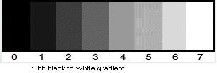
Each intensity value is represented as an 8 bit number. Then there are 256 variation. If the intensity values are represented as 16 bit number, there are 32000 variation between absolute black and pure white.

Fig-1

Representing images in this way however takes a great deal of space. It is difficult to transmit a big file size pictures over limited bandwidth system like internet.
Demand for communication of multimedia data
through the telecommunications network and
accessing the multimedia data through Internet is growing in this days and age[1].With the use of digital
cameras, requirements for storage, manipulation, and
transfer of digital images, has grown rapidly.. Downloading of these files from internet can be very time consuming task. Therefore development of efficient techniques for image compression has become quite necessity [2].
JPEG compression is able to greatly reduce file size with minimum image degradation by eliminate the least important information. But it is considered a lossy image compression technique because the final image is not exactly same with the original image.

2 NEED FOR COMPRESSION

The following example illustrates the need for compression of digital images [3].
a. To store a colour image of a moderate size, e.g.
512×512 pixels, one needs 0.75 MB of disk space.
b. A 35mm digital slide with a resolution of 12μm
requires 18 MB.
c. One second of digital PAL (Phase Alternation Line)
video requires 27 MB.
To store these images, and make them available over
network (e.g. the internet), compression techniques
are needed. Image compression addresses the problem of reducing the amount of data required to represent a digital image. The transformation is applied prior to storage or transmission of the image. At receiver, the compressed image is decompressed to reconstruct the original image

The research paper published by IJSER journal is about A Survey Analysis for lossy image compression using Discrete cosine Transform. 2

ISSN 2229-5518

3. IMAGE DATA REDUNDANCY

Image processing exploits three types of redundancy[4] in image data: coding redundancy, interpixel or spatial redundancy and psycho visual redundancy .
Psycho visual redundancy indicates that some
information in the image is irrelevant and therefore, it is ignored by the human vision system. Coding redundancy is due to the fact that images are usually represented using higher number of bits per pixel than is actually needed. Interpixel redundancy is due to the correlation among neighboring pixels. These characteristics of image data have been identified and exploited in the image compression. The redundancy in image data has not been considered as a potential source for computational redundancy.

4. IMAGE COMPRESSION USING DCT

JPEG is primarily a lossy method of compression. JPEG was designed specifically to discard information that the human eye cannot easily see. Slight changes in color are not perceived well by the human eye, while slight changes in intensity (light and dark) are. Therefore JPEG's lossy encoding tends to be more economical with the gray-scale part of an image and to be more playful with the color. DCT separates images into parts of different frequencies where less
important frequencies are discarded through
quantization and important frequencies are used to retrieve the image during decompression. Compared to other input dependent transforms, DCT has many advantages: (1) It has been implemented in single integrated circuit; (2) It has the ability to pack most information in fewest coefficients; (3) It minimizes the block like appearance called blocking artifact[5], that results when boundaries between sub-images become visible

The forward 2D_DCT transformation is given by the following equation:
……………eq1
where

is the horizontal spatial frequency,
for the integers 0 < u <8.

is the vertical spatial frequency, for

the integers . 0 < v <8 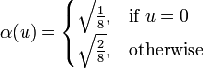is a normalizing scale factor to make the transformation orthonormal
is the pixel value at coordinates
is the DCT coefficient at coordinates

5. JPEG PROCESS STEPS :

Original image is divided into blocks of 8 x 8. Pixel values of a black and white image range
from 0-255 but DCT is designed to work on
pixel values ranging from -128 to 127 .
Therefore each block is modified to work in the range.
Equation(1) is used to calculate DCT matrix. DCT is applied to each block by multiplying
the modified block with DCT matrix on the
left and transpose of DCT matrix on its right.
Each block is then compressed through quantization.
Quantized matrix is then entropy encoded. Compressed image is reconstructed through
reverse process.
This is an example of 8X8 8bit subimage , using matlab code I divide this subimage into 8x8 block which is shown in next picture.

The research paper published by IJSER journal is about A Survey Analysis for lossy image compression using Discrete cosine Transform. 3

ISSN 2229-5518

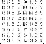
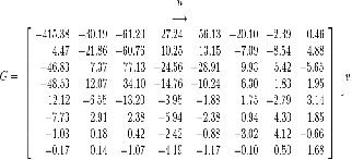
Fig- 3

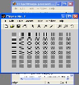
Fig-4 64 two dimensional special frequency

For an 8-bit image, each entry in the original block falls in the range [0,255]. The mid-point of the range (in this case, the value 128) is subtracted from each entry to produce a data range that is centered around zero, so that the modified range is * − 128,127+.

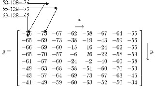
Fig-5

If we perform eq1 on our matrix above, we get the following (rounded to the nearest two digits beyond the decimal point): this is DCT matrix.

Fig-6

Note the top-left corner entry with the rather large magnitude. This is the DC coefficient. The remaining
63 coefficients are called the AC coefficients.

6. QUANTIZATION

Quantization is the step where most of the compression takes place. Quantization makes use of the fact that higher frequency components are less important than low frequency components.. Quantization is achieved by dividing transformed image DCT matrix by the quantization matrix used. Values of the resultant matrix are then rounded off. In the resultant matrix coefficients situated near the upper left corner have lower frequencies .Human eye is more sensitive to lower frequencies .Higher frequencies are discarded. Lower frequencies are used to reconstruct the image[6].
A typical quantization matrix, as specified in the original JPEG Standard, is as follows:

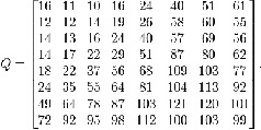
Fig-7

The quantized DCT coefficients are computed with

…………….eq 2

The research paper published by IJSER journal is about A Survey Analysis for lossy image compression using Discrete cosine Transform. 4

ISSN 2229-5518

where G is the unquantized DCT coefficients; Q is the
quantization matrix above; and B is the quantized
DCT coefficients.
Using this quantization matrix with the DCT

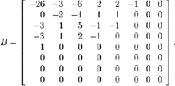
coefficient matrix from above results in:

Fig-8

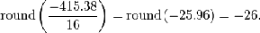
For example, using −415 (the DC coefficient) and
rounding to the nearest integer

7. ENTROPY ENCODING

After quantization, the algorithm is left with blocks of
64 values, many of which are zero.The algorithm uses a zigzag ordered encoding, which collects the high frequency quantized values into long strings of zeros. To perform a zigzag encoding on a block, the algorithm starts at the DC value and begins winding its way down the matrix, as shown in figure 9. This converts an 8 x 8 table into a 1 x 64 vector.

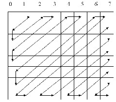
Fig-9 zigzag order encoding

The zigzag sequence for the above quantized coefficients are shown below. (The format shown is just for ease of understanding/viewing.)

−26
−3	0
−3	−2	−6
2	−4	1	−3
1	1	5	1	2
−1	1	−1	2	0	0
0	0	0	−1	−1	0	0
0	0	0	0	0	0	0	0
0	0	0	0	0	0	0
0	0	0	0	0	0
0	0	0	0	0
0	0	0	0
0	0	0
0	0
0

Fig-10
All of the values in each block are encoded in this zigzag order except for the DC value. For all of the other values, there are two symbols that are used to represent the values in the final file. The first symbol is a combination of [S,O] values. The S value is the number of bits needed to represent the second symbol
, while the O value is the number of zeros that precede this Symbol. The second symbol is simply the quantized frequency value, with no special encoding. At the end of each block, the algorithm places an end- of-block sentinel so that the decoder can tell where one block ends and the next begins.
The first symbol, with [S, O] information, is encoded using Huffman coding. Huffman coding scans the data being written and assigns fewer bits to frequently
occurring data, and more bits to infrequently occurring data. Thus, if a certain values of S and O happen often, they may be represented with only a couple of bits each. There will then be a lookup table that converts the two bits to their entire value. JPEG allows the algorithm to use a standard Huffman table, and also allows for custom tables by providing a field in the file that will hold the Huffman table.

The research paper published by IJSER journal is about A Survey Analysis for lossy image compression using Discrete cosine Transform. 5

ISSN 2229-5518

DC values use delta encoding, which means that each
DC value is compared to the previous value, in zigzag
order. Note that comparing DC values is done on a
block by block basis, and does not consider any other data within a block. This is the only instance where blocks are not treated independently from each other. The difference between the current DC value and the previous value is all that is included in the file. When storing the DC values, JPEG includes a size field and then the actual DC delta value. So if the difference between two adjacent DC values is –4, JPEG will store the size 3, since -4 requires 3 bits. Then, the actual binary value 100 is stored. The S field for DC values is included in the Huffman coding for the other S values, so that JPEG can achieve even higher compression of the data.

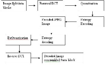
9. BLOCK DIAGRAM OF ENCODING AND DECODING PROCESS

8. DECOMPRESSION

Decompressing[8] a JPEG image is basically the same as performing the compression steps in reverse, and in the opposite order. It begins by retrieving the Huffman tables from the image and decompressing
the Huffman tokens in the image. Next, it
decompresses the DCT values for each block, since
they will be the first things needed to decompress a
block. JPEG then decompresses the other 63 values in each block, filling in the appropriate number of zeros where appropriate. The last step in reversing phase four is decoding the zigzag order and recreate the 8 x
8 blocks that were originally used to compress the

10. RESULT

Fig-11

image.
The IDCT takes each value in the spatial domain and
examines the contributions that each of the 64
frequency values make to that pixel.

In many cases, decompressing a JPEG image must be done more quickly than compressing the original image. Faster implementations incur some quality loss in the image, and it is up to the programmer to decide which implementation is appropriate for the particular situation. Below equation shows the equation for the inverse discrete cosine transform function.

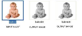
fig 1 fig 2 fig 3
The input image shown in fig.1 to which the DCT algorithm is applied for the generation of codes and then decompression algorithm(i.e. DCT decoding) is applied to get the original image back from the generated codes, which is shown in the Fig.3.The size of original image differ with the output image(fig 2)i.e compressed image. The compression ratio is the ratio of original size / encoding image size
So Compression ratio =7.47/7.27=1.024 and The size
of output image i.e decompressed image is the 7.07

f x, y

1 7 7

C u C v F u, v cos 2x 1 u

cos 2 y 1 v

from the Fig.3 it is clear that the decompressed image

4 x 0 y 0 16

………….eq 3

16 is not equal to the input image. Image will be sort of

lossy type, and quality also differ with the original
image.

The research paper published by IJSER journal is about A Survey Analysis for lossy image compression using Discrete cosine Transform. 6

ISSN 2229-5518

11 . CONCLUSION

The experiment shows that the compression ratio achieved by applied discrete cosine transformation algorithm is not so good. The above presented a compression and decompression technique based on dct encoding and decoding method for scan testing to reduce test data volume, test application time is actually a survey Experimental results show that up to a 1.024 compression ratio for the above image .we conclude that dct method of image compression is efficient but lossy technique for image compression
and decompression to some extent. As the future work on compression of images for storing and transmitting images can be done by other lossless methods of
image compression because as I have concluded that
the above result of decompressed image is not almost
same as that of the input image so that indicates that there is some loss of information during transmission.

I2. REFERENCE

[1.] Digital Compression and Coding of Continuous tone Still Images, Part 1, Requirements and
Guidelines. ISO/IEC JTC1 Draft International Standard
109181, Nov. 1991.
[2.] Greg Ames, "Image Compression", Dec 07, 2002. [3] Compression Using Fractional Fourier Transform A
Thesis Submitted in the partial fulfillment of requirement for the award of the degree of Master of Engineering In Electronics and Communication. By Parvinder Kaur.
[4] Rafael C. Gonzalez and Richard E. Woods. Digital

Image Processing. Prentice Hall, 2008.

[5.] ken cabeen and Peter Gent, "Image Compression and the Descrete Cosine Transform "Math 45,College of the Redwoods.
[6]. Hudson, G.P., Yasuda, H., and Sebestyén, I. The international standardization of a still picture compression technique. In Proceedings of the IEEE Global Telecommunications Conference,IEEE Communications Society, Nov. 1988, pp. 10161021.
[7] David Jeff Jackson and Sidney Jwl Hannah “Comparative analysis of image compression technique” Department of Electrical Engineering ,The University of Alabama, Tuscaloosa, AL 35487.This paper appears in system theory 1993,proceeding SSSST’93, twenty fifth edition southeastern symposium on 9 th march 1993 on pages 513-517.
[8] G. K. Wallace, 'The JPEG Still Picture Compression
Standard', Communications of the ACM, Vol. 34, Issue
4, pp.30-44.