International Journal of Scientific & Engineering Research Volume 4, Issue 2, February-2013 1

ISSN 2229-5518

On the Kinematics of Hyper Redundant Mobile

Robot

Dilip Kumar Biswas, Subhasish Bhaumik, Jyotirmoy Saha

Abstract— The kinematics of any ‘n’ DOF hyper redundant mobile robot of interconnected links is considered for this analysis. The kinematic configuration facilitates to find out the joint parameter. Precise calculations decide the closeness of the actual consideration of every kinematic configuration. Only the centre line of the robot is considered for this analysis. The existence of acceptable free space conform the alignment chord, termed as backbone curve, which resemble the chain of interconnected links. The kinematics of the robot in free space is defined by the Denavit and Hertenberg principle. In our analysis each link has two joints and all the joints have the ability to pass through the backbone curve. To find the existence of each joint on the backbone curve we construct a Cardinal Spline in between two consecutive path points on the backbone curve and on this spline a large number of points are constructed. We use error minimization strategy to evaluate the position of all the joints except the frontal one which is the end of the virtual link and its position is obtained by the path points. Each pair of joints results the pose information of that segment. The proposed algorithm is validated through computer simulation.

Index Terms— Kinematics, Redundant, D-H Parameter, Cardinal Spline, Pose Variants, Potential Field, Constraints.

——————————  ——————————

1 INTRODUCTION

N autonomous intelligent robotic vehicle navigates through its predefined known workspace to perform varieties of tasks in many stations without intervention
of human operator require a well accepted, fast, optimal and on line navigation algorithm that can perform efficiently and effectively[1]. The robot plan its action as per the feedback obtained from the environment depending on practical con- straint. The planning is function or task specific and track or path specific. The task is predefined or autonomous as per the requirement and stationary but the path is environment de- pendent and target oriented. Planning of task is easy but path planning necessitates collision free space towards the target or task field that has acceptable cost in terms of time, energy and distance. A mobile autonomous robot, targeted from one sta- tion/start point to another station/goal point in an environ- ment, plans a feasible path avoiding obstacles in its way and satisfies the criterion of autonomy requirements such as: ener- gy, time, and safety. As a result, the foremost mission for path planning of autonomous mobile robot is to explore a realistic collision free path.
Path planning is the basic requirement of a mobile autono- mous vehicle [2,3,4,5]. This is a pretty simple problem but not so easy to result a desired outlay. The path so obtained must be free from obstacles. The complexity may accumulate with the increase of number of considerable constraints such as path-planning, obstacle avoidance, kinematics, dynamics and uncertainty. These considerations make the problem an active research area.

————————————————

 Dilip Kumar Biswas is currently pursuing PhD in Legged Robotics in Jadavpur University, India, PH-03436452046. E-mail: dbiswas@cmeri.res.in

 Subhasish Bhaumik is Professor and guide from BESU, Howrah, India, E-

mail: sbhaumik_besu@yahoo.co.in

 Jyotirmoy Saha is Professor and guide from JU, Kolkata, India, E-mail:

jmoysaha@yahoo.co.in
The configuration space, Cspace, [5,6,7,8] of a planner robot moving on a plane has the same dimension as the work space but for a complex robot, the dimension of the configuration space is higher. If the space is free from obstacles it is Cfree and occupied by obstacles it is Cobs or forbidden space. At the boundary of the obstacles both are present and the movement of the robot along (as close as possible) the boundary termed as ‘wall following’. This implies that the work space of the mobile robot is throughout the free space, Cfree and extended till boundaries of the Cobs or forbidden zone.
The autonomous and intelligent mobile robot is an intelli- gent mobile machine [1,6,7] which is capable to function in a structured or unstructured, lightly or densely cluttered envi- ronment. A fully equipped self autonomy robotic system re- quires intelligent components for interaction with the envi- ronment and parallel computing platform to compute the functional algorithm quickly. The autonomous and intelligent robot decides intelligently to find out a feasible collision free path during movement in the workspace. The path planning algorithms [5,6,7] guide the robot along the generated trajecto- ry in the Cfree zone satisfying implied holonomic or non- holonomic vehicle constraints. This guiding methodology drive the vehicle to satisfy the reachability criteria from initial pose to the final pose maintaining configuration space barrier. To maintain the poses a non-holonomic vehicle may require long path but holonomic vehicle, for its intrinsic kinematic constrains, can behave instantly. So the spot rotation, whatev- er we are habituated to listen for non-holonomic vehicle is almost imaginary and practically to get it is very difficult.
The robotic researchers across the world are engaged on this topic and various works are reported till date. The fast and feasible on-line path planning algorithm is still under ex- ploration and the path planning algorithms are limited to points robot but the robot has any arbitrary shapes and obsta-

International Journal of Scientific & Engineering Research Volume 4, Issue 2, February-2013 2

ISSN 2229-5518

cles has complicated texture, this leads the planning algorithm very complicated and time consuming. In this work a physical geometric figure has been considered which has same project- ed size on 2D workspace. Moreover the robot which has been considered here is a multi-section modular structure. This means that the robot is a long chain of similar building blocks with ability to carry various payloads in different module. This let the robot to carry all type of required intelligent com- ponents as well as power packs for extra area coverage and extra working time.
A collision free path planning strategy is essentially require to realize the autonomous motion of a mobile robot through work space populated with obstacles. Various techniques such as Visibility Graph, Voronoi Diagram, Cell Decomposition, Behavior Based Model, Genetic Algorithm [6,7,9] etc are very much fruitful to search for the free space in the environment. All the methods are ‘off-line’ and check whether the goal is reachable or not prior to start moving. Path planning of modu- lar robot is difficult in the sense that the robot itself is a chain of interconnected robots. Path planning for a single section robotic body and multi-section robotic body is completely dif- ferent. As the system is a chain of segments the speed of each segment is same but the velocities are different. The path of the first segment is followed by other segments and thus the first segment is assigned as master and other segments are assigned as follower. Potential Field algorithm is chosen and tested finding suitability and ease of application. The potential field method is simple, fast and can be utilized on-line plan- ning. It has good potential for decision making characteristic and always targeted towards the goal. Many researchers are using this algorithm for its fast, low cost, real time and feasible solution. Path planning of modular robotic system is depend- ent on segmental pose of any segment with the preceding and succeeding segments. Here we have limited the segmental pose which is basically the segmental orientation to a certain degree. This can vary as per the functional requirements as well as environmental relationships of the system.
The modular robot should have the ability to perform as per the requirement and can take decisions independently to avoid collision with any unwanted perturbation which has appeared in its path. In each step of planning, the robot con- siders the environment as static and forgets all the conditions at the next moment. It starts again to examine the surround- ings as well as the goal to react in the next moment and con- siders the environment again to cope up from any undesirable situation. Therefore it seems that this path planning algorithm may be applicable in real time obstacle avoidance.
In the unknown environment the robot is awaiting for the information of existence of the next predicted point to trav- erse. A series of path points generated during the course of action and presently the CG of the robot passing through the generated path. The tracking method is also interesting. Each of the generated predicted points, which are existing, is target- ed as soon as the robot reaches its current location. For a sin- gle segmented wheeled or legged robot this technique of path
following is considered and all the related calculations are also faced with CG technique. But in case of a multi segment robot CG guided path tracking fails instead back bone guiding methodologies are adopted which follows the Active Chord Mechanism (ACM). In which the main consideration of seg- mental pose is the frontal and rear joints should pass through the path curve. For this doctrine at any instant the joints must lie on the back bone as well as the path curve and the pose/orientation of any segment depends only on the path points, which are stepwise the on-line or off-line path posi- tions. This is very important because the points present in this connection must be spread throughout the whole body length of the modular robot. The kinematic configuration of any modular robot at any instant depends on the back bone curve generated by path points.

2 THE CONFIGURATION KINEMATICS

The robot has many segments, for our analysis a seven segmented robot has considered, a 3D CAD model of which is shown in figure-1. The robot is holonomic by configuration. Every segment consists of four insect type legs. Each leg has three degree of freedom. Three motors are used to drive the leg. The intermediate segment has two universal joints passing through the configuration curve obtained from path infor- mation, figure-2. But these universal joints do not have any actuator to drive. They are inactive joints. For ease of our analysis only the centre lines of all the segments are consid- ered, which means that the robot is an assembly of piecewise straight line. The two end points of every line are intercon- nected except the forward and tail one so that it can form an open chain kinematic structure. As a whole this kinematic structure confirms six DOF spatial configurations. This spatial kinematic configuration of the robot is structured by back bone curve. All the end points of each of the segmental straight lines pass through the back bone curve. The front junction is obtainedfrom the kinematic parameter of D-H con- vention and other junction points and tail is obtained by the proposed method those are always passing through the path curve.

Fig. 1. The General assembly of 3D CAD model of the proposed Hy- per Redundant Legged Mobile Robot (7DOF).

International Journal of Scientific & Engineering Research Volume 4, Issue 2, February-2013 3

ISSN 2229-5518

the considered kinematic pose is shown in figure-4.

Actual Links

y2 y3 y4 y5

3

y8 9

8

7

Tail

Virtual Links

Head

5 6

4

1

Fig 4. Kinematic configurations of 7 DOF robot moving in 2D plane

TABLE 1

D-H PARAMETER FOR n NUMBER OF LINK CHAIN

i θi αi ai di

Fig. 2. The 3D CAD model of an intermediate single module showing the joints to connect with other modules

Actual robot kinematics

1 θ1 α1 a1 d1

2 θ2 α2 a2 d2

3 θ3 α3 a3 d3

4 θ4 α4 a4 d4

5 θ5 α5 a5 d5

……………………………………………………………..

i θi αi ai di

y y3

yiii yn 

……………………………………………………………..

2 3 4 5 iii+1

n+1

n θn αn an dn

o2 x2 o3

2

x3 o4 x4

oiii

xiii

Where: i is the link number, θi joint angle, αi joint twist angle ai link offset and di joint offset

Virtual Links and

 cosθi
-cosα i sinθi
sinα isinθi
a icosθi 

joints  

Z i -1 T =  sinθi

cosα i cosθi
-sinα icosθi
a isinθi 

(1)

Y0 

i  

1 i

X  

O0 0  

Fig 3. Generalized kinematic configurations of proposed multi- segmented robot in 2D moving on a simplified plane.

The kinematic representation of the robot has two part, vir- tual links and real robot as shown in the figure-3. The D-H table so obtained is specified in table-1. Virtual links connect the robot with the global frame. The virtual link attached with the global reference frame has at least one rotational joint and only one translational joint, Figure-3. The virtual link attached to the robot must have at least one rotational joint. The robot

3 FINDING JOINT ANGLES

3.1 The Cardinal Spline

For local interpolation splines are used from long back. Cardinal Spline [14] is a generalized form of Catmull-Rom spline and general third order parametric spline [10,11,12,13,15] can be represented in matrix form as follows.

 a1 

 

working in 2D workspace comprises of many segments and
each segment is interconnected with no less than one rotation-

X (  )    3  2 

1 . a2 

 a 

(2)

al joint at each end. So finally the basic kinematic configura-  3 

tion of the said robot comprises of many segments of straight lines. We restrict our analysis further in 2D environment and

a4 

Where ρ is bounded as; 0 ≤ ρ ≤ 1.

International Journal of Scientific & Engineering Research Volume 4, Issue 2, February-2013 4

ISSN 2229-5518

Fig. 5. Control points and the Gradients

The coefficients a1,a2,a3 and a4 are different in each section of the Cardinal Spline and need to be determined, considering the boundary conditions X(0) and X(1), and considering re- quired continuity (tangent continuity) at the extreme points. Each segment of Cardinal Spline uses four consecutive control points to set the boundary condition. The gradient at Xk is the gradient of the line connected Xk-1 and Xk+1. Similarly the gra- dient at Xk+1 is the gradient of the line passing through the control points Xk and Xk+2, figure-4. Thus the result of the curve segment so formed by the four control points is connect- ing the intermediate two points, whereas at the starting and ending, control points give the continuity at the intermediate points.
Thus equation (2) can be expressed as

 X k 1 

 

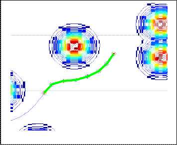
step size between (n-k)th and (n-k-1)th path points be Sn-k. It is to be noted that the relation between segmental length and the maximum step size become ds>(Sn-k)max, Fig-7. In any instan- taneous step the head i.e. the frontal point of the foremost segment or end effector of the virtual link, follows each of the step position. But where will be the position of other joints and the tail? To find these locations we considered intersection points of circle of radius ‘ds’ and the Cardinal Spline connect- ed by two closest path points of the boundary of the circle. The intersection between the set of path points and the circle is considered as internal points of the circle and all other path points are external points. Out of all the internal points maxi- mum two are closest to the periphery of the circle and out of all the external points maximum two are closest to the outside of the circle. There are two sets of points so formed are either side of the circle and each sets of points are closely spaced. Out of these two sets of points one set is already considered for calculation of positional information of the previous joints so only one set of boundary points are left for finding the in- tersection points of the considered segment, which will lead the joint location. Let the ith circle is centered in joint Ji and the valid boundary path points found out from the generated points of Cardinal Spline, and they are (n-m)th and (n-m-1)th. To form cardinal Spline between (n-m)th and (n-m-1)th points at any instant we select four consecutive points like (n-m+1)th, (n-m)th, (n-m-1)th and (n-m-2)th points. In each step the back bone curve changed depending on the positional information calculated from this methodology. The segmental poses de- pend on the positional and orientation information of each segment on the back bone curve.

X ( )   3  2

 1 .C

.  X k 

(3)

  M

 X k 1 

 

 X k 2 

Where, CM is the cardinal matrix and obtained as

s

2  s s  2 s 

 2s s  3 3  2s

s 

(4)

  

M s 0

s 0 

 0 1 0 0 

and s is defined as

s  1 (1  t)

(5)

The value of ‘t’ i.e. the tension parameter conform the looseness or tightness of the curve passing through the control points maintaining desired continuity at each junction.

3.2 Finding Joint Positions

To find the positional information of each segmental joint as well as the tail and head we have adopted a very lucid and easy method. With reference to the figure-6 considering the equal segmental length throughout the body be ‘ds’ and the

Fig. 6. Instantaneous segment circles and the path points

3.3 Angle between two consecutive Segment

From simple geometric relation the slope of line connecting points (i-1) and i be,

International Journal of Scientific & Engineering Research Volume 4, Issue 2, February-2013 5

ISSN 2229-5518

m(i 1)i

 yi 1  yi

xi 1  xi

(6)

sen as per the information of the following table-2,

TABLE 2

CONDITION FOR HEADING ANGLE

The included angle between two consecutive straight lines as shown in figure-8, be,

tan i

 m(i 1)i  mi (i 1)

1  m(i 1)i mi (i 1)

(7)

Where ø is the included angle between two successive segments.

3.4 The kinematic Equations

Transformation of each segment is obtained by the coordi- nate transformation matrices. The robot itself is a serially con- nected links and the pose of each link is determined by the following taansformation matrics.
The DH transformation matrix for first link by equation(1)

Fig. 7. Instantaneous segmental pose of a modular robot and the

cos1

 cos 1 sin 1

sin 1 sin 1

a1 cos1 

generated path points  

0  sin 1

cos 1 cos1

 sin 1 cos1

a1 sin 1 

 0 sin 1

cos 1

d1 

 0 0 0 1 

 

i

i cos1

0  sin 1 0

m(i-1)i  

i

m(i-1)i

  si



 (9)

0

1

 

(i-1)

Fig. 8. Joint angle between two segments

3.4 Logical selection of joint angle

Let us define the following
Similarly 1T2, 2T3, 3T4, 4T5, 5T6, 6T7, 7T8, and 8T9 can be evalu- ated by using equation (1).
Therefore the transformation matrics for other links in re- spect to the base frame are as follows-

0 T = 0 T 1 T

2 1 2

0 T = 0 T 2 T

Pi 1Pi  ( xi  xi 1 )( yi  yi i ) 

3 2 3

0 0 3

   

T4 = T3 T4

Pi 1Pi 1

( xi 1

xi 1 )( yi 1

yi 1 )



0 T = 0 T 4 T

Pi Pi 1  ( xi  xi 1 )( yi  yi 1 ) 

(8)

5 4 5

0 0 5

(10)

   

T6 = T5 T6

Pi 1Pi Pi 1

2( xi

xi 1 )( yi 1

yi 1 )

0 T = 0 T 6 T

Pi 1  Pi 1P  Pi P  Pi 1Pi Pi 1 

7 6 7

0 0 7

Where (x, y) are the coordinate of the end points of central axis of each segment. These parameters help us to determine the actual joint angle at any configuration. The ’s will be cho-

T8 = T7 T8

0 T = 0 T 8 T

9 8 9

International Journal of Scientific & Engineering Research Volume 4, Issue 2, February-2013 6

ISSN 2229-5518

4 SIMULATION

It is to be noted that offline planning is possible only in the static environment but if the environment itself is dynamic the question of offline planning is imaginary. Moreover an auton- omous mobile robotic system requires on line path planning to fulfil its esteemed title. A robot is said to be autonomous if all of its mobile characteristics has the ability to take independent decision by own at any time. Any system with autonomous ability does not result an optimum path but they assure non collision with the mobile or static obstacles, Fig-9 and Fig-10. The planning algorithm so chosen must have inherent simplic- ity and leads least computational burden. In real time problem any animal traverse its desired goal and from its own intelli- gence and they overcome from any unwanted situation. In our work we consider only the kinematic part that basically fol- lows the obstacle free space which is decided by the path planning algorithm. The kinematic configuration so formed for the modular robot has least computational complexity.
bratory path. The algorithm so developed is uniquely applica- ble to holonomic robot like legged robot. To utilize this for nonholonomic robot the algorithm has to be changed accord- ingly, where only the midpoint of the two end points of the robot may need to be found out with other parameters.

Movement of the MODULAR Robot

TARGET

Fig. 10. An enlaged view of obstacle avoidance of modular robot

(a)

10 10

START

-10

0 5 10 15 20 25 30 35

Global X-Axis

Fig. 8. Obstacle avoidance of the modular robot

In our present kinematic configuration the robot’s frontal point follows the path planning decisions but the joints and rear point are computed on the basis of circle and Cardinal Spline intersection. But the exact solution is not found out so apply the theory of approximation. This results an approxi- mate solution that is closest to the exact solution.
It is to be noted that the robot is a quasi-rigid link of finite length with compliant leg. Obstacle avoidance is easy in light- ly cluttered environment. The robot has an initial and final station those maintain continuity and for our robot these sta- tion are the segments of circular path.
The robot rotates instantaneously in an amount of absolute

-20

-1

-2

-3

-4

0 100 200 300 400 500 600

Number of steps

(b)

0 100 200 300 400 500 600

Number of steps

heading angle to align itself towards the next predicted posi- tion. From analysis it is shown that the fluctuation of change of heading angle is more in present method comparing to the proposed method as shown in figure-11. The present method leads huge angular deviation that leads the velocity and accel- eration in proportion to the huge change of heading angle in comparison to the angular velocity and acceleration of the proposed method. It is also to be noted that due to less varia- tion of angular rotation the robot leads a smooth and less vi-

Fig. 10. Fluctuation of heading angle in each instant (a) Heading an-

gle of a point robot same as the CG of the first module passes through path points, (b) Heading angle while the frontal joint of the first module passes through path points and rear joint passes through the intersection point

5. DISCUSSION

The robot is considered as a multi-section/ modular mobile robot. Each module has same dimension along the central axis.

International Journal of Scientific & Engineering Research Volume 4, Issue 2, February-2013 7

ISSN 2229-5518

The consecutive two modules are connected via a universal joint (as shown in the figure2) and termed as junction. In front of the front module there are navigational sensors and at the both sides along the central axis there are proximity sensors and the means of locomotion are considered to be attached at suitable positions of each module. Each junction and front and rear points of the front and rear modules have to pass through the path so generated by the planning algorithm. Each module has some flexibility to impart springing action to accommo- date the compliance characteristics of the robot and this is achieved by the coupler of the joints.
Online path planning of this robot in an unstructured un- known environment is a difficult task. The computations re- lated to the robot is much higher compare to point robot and if the path planning algorithm is little complicated then the total computation time required will be more which may lead colli- sion instead of avoidance. The obstacle may come closer be- fore the end of single step computation of taking decision.
It is to be noted that the robot is a long chain of rigid links. The avoidance is possible only for the frontal module and all other modules are the follower of the first module so the first module is termed as master and others are follower. If any- thing collide with the later sections laterally it is not possible to avoid by the present algorithm. But once the obstacle is avoided by the front module and if the obstacles are mobile and intelligent enough then there is no chance of collision. The robot has an initial and final station those maintain the tangent continuity always and for our robot these station are the seg- ment of a circular path.

6. SCOPE FOR FUTURE WORK

The methods are simple and the computational complexity is less so, they can be used in wheeled or legged modular ro- bots for implementations.
Only the body segments are considered in the present work the locomotors will be considered in future work.
Dynamic properties of the robot are not considered in the present work, which will be considered in future study.
Only 2-D workspace is considered in the present work but in future, an attempt will be made to consider a 3-D work- space.

7. CONCLUDING REMARKS

Modular multisectional robot comprised of many intercon- nected modules forming as serially connected link structure. Computationally fast and elegant path planning algorithm is the only choice for online navigation of this robot. Kinematics is the deciding factor for pose variation. Finding the pose in each stepping movement require huge optimization that slow- ing the movement due to demand of huge computation. In this analysis we have a novel curve fitting method that finds out the positional information of every intersection of each module of the modular robot. Present scenario is such that the robot’s CG passes through every step position and heading angle is calculated separately. But our analysis does not re- quire any optimization and calculation for heading angle. These reduce the computation time drastically and favoured
to online path planning. This method is not only applicable in modular robot but also can be used in any mobile robot to solve online as well as offline path planning problem. To uti- lize its elegance it requires a problem free and fast responding path planning algorithm. To judge its utility the path plan- ning problems of modular multisection robots working in a
2D workspace have been solved using the principle of cardinal spline and potential field method. The performance of both the approaches depends on the nature of the functions used. As the potential field approach is found to be computationally not so complex, it can be used for on-line implementations where as the cardinal spline approach results a smooth path and suitable for off-line planning for its simplicity and ele- gance. Cardinal spline may also be applicable on-line in a workspace with few numbers of obstacles.

REFERENCES

[1] J.L. Crowley, Navigation for an Intelligent Mobile Robot. IEEE journal of robotics and automation, vol. RA-I, No. 1, 1985

[2] Jiang, Seneviratne, Earles., (1997).Time-optimal smooth-path motion plan- ning for a mobile robot with kinematic constraints. Robotica, Vol. 15, pp. 547–

553.

[3] Murray, Sastry., (May 1993). Nonholonomic Motion Planning: Steering Using

Sinusoids. IEEE Transactions on Automatic Control, vol. 38, No. 5,.

[4] Lacroix, Fleury, et al., (1998). Reactive Navigation in Outdoor Environments.

IJRR special issue on ‘Field and Service Robotics’.

[5] Ippoliti, G., Jetto, L., Longhi, s. (2005). Localization of mobile robots: Devel- opment and Comparative Evaluation of Algorithms Based on Odometric and Inertial Sensors. Wiley InterScience – Journal of Robotic System, vol. 22, no. 12, pp. 725-735.

[6] Howie Choset et al., Principles of Robot Motion—Theory, Algorithms, and

Implementation, The MIT Press, 2005.

[7] Jean Claude Latombe., Robot Motion Planning, Kluwer Academic Press,

1991.

[8] Hsu, Latombe and Motwani., Path planning in expansive configuration

Space, Int. Journal of Computational Geometry & Applications, Vol. 9, No.

4&5, pp. 495-512, 1999.

[9] Masehian, Amin-Naseri., A voronoi diagram-visibility graph-potential field compound algorithm for robot path planning, Journal of. Robotic Systems, Vol. 21, No. 6, pp. 275–300, 2004.

[10] Halit Eren, Chun Che et all., Implementation of the Spline Method for Mobile

Robot Path Control, IEEE, p. 739-744, 1999.

[11] Figueiredo, R. J. P.; Markandey, V., Spline based algorithms for shape from shading (for robot vision application), Proceedings of the SPIE, The Interna- tional Society for Optical Engineering, Vol. 850, p. 152-5, 1988.

[12] W. Boehm, Multivariate spline algorithms, Mathematics of Surfaces. Proceed- ings of a Conference. Clarendon Press, Oxford, UK, 1986, 197-215.

[13] H. Spath, A. K. Peters, Wellesley, One Dimensional Spline Interpolation Algo- rithms, Massachusetts, 1999

[14] D. K. Biswas, Spline Guided Path of a Mobile Robot with Obstacle Avoidance Characteristics, 14th National Conference on Machines and Mechanisms (NaCoMM-09), Dec 2009, 266-271.

[15] Laumond., Feasible trajectories for mobile robots with kinematic and envi- ronment constraints, Intelligent Autonomous Systems, Dec-1986, 346-354.

[16] O. Khatib., Real-time Obstacle Avoidance for Manipulators and Mobile Ro- bots, International Journal of Robotics Research, 5(1), 1986, 90-98.

International Journal of Scientific & Engineering Research Volume 4, Issue 2, February-2013 8

ISSN 2229-5518

[17] Valavanis, Hebert, et al., “Mobile Robot Navigation in 2-D Dynamic Environments Using an Electrostatic Potential Field,” IEEE Transac- tions on Systems, Man, And Cybernetics—Part A: Systems and Hu- mans, 30(2) , March 2000, 187-196.

[18] Beard, T.W. McLain., “Motion Planning Using Potential Fields,” Brigham

Young University, Provo, Utah 84602, January 2003.

[19] Lin, Kuo, & Chuang., Potential-Based Path Planning for Robot Manipulators, Journal of Robotic Systems, 22(6) , 2005, 313–322.

[20] Horn, The fundamental ell equation, Technical report, Working paper no. 116, Artificial Intelligence Laboratory, MIT, Dec. 1975.

[21] S. Hirose, & A. Morishima, Design and control of a mobile robot with an articulated body, International Journal of Robotics Research, 9(2), 1990, 99-114.

Dilip Kumar Biswas is a Ph.D student of Jadavpur University. He received his BE(Mech Engg) from REC Durgapur and M.Tech(Design and Production Engg) from NIT Durgapur in 1994 and 2004 respec- tively. Presently he is working as scientist at CMERI Durgapur. He published 13 research papers. He re- ceived CSIR technology award 2003 along with his project team members. He was engaged in R&D activ- ities as Leader in 4 research projects and as member in another 5 research projects. Presently he is engaged in one research project and subsequently proposed an-

other two research works. His research interest are Machine Design and Robotics

particularly Mobile Robotics. He is a member of the Institution of Engineers

(India) and life member of Association for Machines and Mechanisms (AMM).

Dr Subhasis Bhaumik received his B.E. (Mechanical) from North Bengal University in 1990, M.Prod.E. (Pro- duction) and Ph.D (Robotics) from Jadavpur University Kolkata in 1992 and 1996 respectively. He served as Re- search Associate in Tata Steel - Jadavpur University joint research project in the area of robotics. He served as facul- ty in BIT Mesra, TIET Patiala, REC Durgapur and BESU Shibpur Howrah. He is also serving as coordinator, School of Mechatronics & Robotics. He has carried out research projects funded by Indo-US Centre for Research Excel- lence in Fabrionics (IUCREF), Board of Research in Nu-

clear Science(BRNS), DST (SERC), AICTE (R&D and RPS), UGC and Larsen &

Toubro Limited (L&T). He has published papers, guided M.tech and Ph.D thesis, written book chapters for In-Tech Austria and Springer-Verlag and received AIMTDR best paper award. His research interests include multi-fingered dexter- ous hands, bio-mimetic robotic systems, mechatronics, mobile vehicles and indus- trial automation.

works for Industry.

Dr J. Saha received his PhD degree from Jadavpur Univer- sity at Kolkata. He is currently a Professor at the Depart- ment of Production Engineering of Jadavpur University. He has published more than 50 research papers in the area of Manufacturing and related areas. His research interests are, Application of CAD-CAM in manufacturing, Robotics, Flexible Manufacturing System, Vibration in Machine Tools, Non-Traditional Machining. He has been joint au- thor of 3 books. He is a member of the Institution of Engi- neers (India). He has also carried out few consultancy